
Macro II Moed B 2025 — Worked Solutions
- #macro-economics-ii
- #past-paper
- #worked-solution
- #multiple-choice
- #classical-theory
- #solow
- #is-lm
- #mundell-fleming
- #phillips-curve
Macro II Moed B 2025 — Worked Solutions
Part of: Macro-Economics II Moed B, 17 March 2025 — Intermediate Macroeconomics (6827), Dr. Alon Cohen. 25 multiple-choice questions, 4% each, open notes, 2.5 hours. Builds on: Lec_03-Classical Theory & National Income · Lec_04-The Monetary System · Lec_05-Inflation · Lec_06-AS-AD Model & Economic Fluctuations · Lec_07-Aggregate Demand I & the IS-LM Model · Lec_08-Aggregate Demand II & Applying the IS-LM Model · Lec_09-The Open Economy Revisited & Mundell-Fleming Model · Lec_14-Aggregate Supply & the Phillips Curve
Which sitting is this?The PDF header says "Moed A, March 17th, 2025", but 17 March is the Moed B (March) sitting. The other 2025 paper (
2025 Moed A Tofes 0) is the earlier sitting. This note is Moed B.
AI-solved questions: ALL 25 (Q1 to Q25)This is a tofes 0 paper and there is no official key. Every answer below was solved independently by me first, then compared with option A (the tofes 0 convention: the official answer is printed first before the options are shuffled). My independent solution agreed with option A on all 25 questions. Not official. Check before relying on them. Questions outside the lecture notes (the Solow and endogenous growth questions, Q6 to Q9 and Q16) are answered from the standard Solow model and the cheat sheet, since Ch 8-9 has no lecture deck.
The questions are shuffled, so the printed letters mean nothingIn the exam the options are reshuffled per student. Below, "A" always means the option printed first on this tofes 0 paper. Q11, Q13 and Q17 refer to graphs that are missing from the PDF. They are embedded in the
.docxversion of the same paper, and are reproduced here.
What this paper tests
The paper in one paragraphA cleaner, more conceptual paper than most: lots of one-line theory questions, a few calculations.
- Classical theory and money (Q1, Q2, Q3, Q4, Q5): real wage from the marginal product of labour, loanable funds, quantity theory, the Fisher effect and an announced money growth path, the classical dichotomy.
- Growth (Q6 to Q9, Q16): above the golden rule, endogenous growth, golden-rule saving rate equals capital share, steady-state .
- AS-AD (Q10, Q11, Q12): demand shocks, the self-correcting path back to , central banks accommodating an oil shock.
- Keynesian cross and IS-LM (Q13, Q14, Q15, Q17, Q18, Q19): inventory adjustment, LM slope, tax vs spending multiplier, holding constant, solving an IS-LM system.
- Mundell-Fleming (Q20, Q21, Q22): perfect capital mobility, floating vs fixed.
- Phillips curve (Q23, Q24, Q25): the trade-off, expectations shifts, a calculation.
Q16 and Q19 are the only numerical IS-LM/Solow ones; Q3 and Q25 are quick arithmetic.
Q1 — What raises the real wage
AI-written answer, consistent with the tofes 0 layout (answer printed first).
Question. In the Classic Theory, the real wage will increase if:
- A. the productivity of labor increases.
- B. the supply of labor increases.
- C. the price of output increases.
- D. the supply of capital decreases.
Answer: A
In the classical model firms hire labour until the real wage equals the Marginal Product of labour, . Anything that raises raises the real wage. See Production Function and Lec_03-Classical Theory & National Income.
- B. False. More labour supply moves along the same curve (diminishing returns), so falls.
- C. False. The real wage is already net of . A higher raises the nominal wage proportionally and leaves unchanged.
- D. False. With less capital, each worker has less to work with, so falls and so does the real wage.
🗣️ In plain EnglishWorkers get paid what an extra worker produces, so the real wage rises when workers become more productive. More workers or less capital pushes it down.
Q2 — Technology shock to investment demand
AI-written answer, consistent with the tofes 0 layout (answer printed first).
Question. In the Classic Theory, when there is a technological advance that leads to an increase in investment demand:
- A. investment is unchanged and the interest rate rises.
- B. investment increases and the interest rate rises.
- C. investment and the interest rate are both unchanged.
- D. investment increases and the interest rate falls.
Answer: A
Classical supply of loanable funds is national saving . With fixed and , unchanged, saving is a vertical line. Higher investment demand shifts the curve right, so the whole adjustment is in the interest rate. In equilibrium , and did not move. See Loanable Funds Market, National Saving and Real Interest Rate.
- B. False. can only rise if saving rises, and it does not.
- C. False. Demand for funds rose, so the price of funds () must rise.
- D. False. A rightward shift of demand cannot lower the price.
IntuitionThe extra demand for funds just bids up , which crowds out the extra investment that firms wanted. See Crowding Out.
🗣️ In plain EnglishFirms want to invest more, but the pool of saving is fixed. So the interest rate rises and the actual amount invested stays put.
Q3 — Quantity theory and velocity
AI-written answer, consistent with the tofes 0 layout (answer printed first).
Question. Consider the Quantity Theory. If the money supply is growing at a 10 percent rate, real output is growing at a 3 percent rate and the average inflation rate in this economy is 7%, then the velocity of money ________.
- A. is constant
- B. decreases
- C. increases
- D. is 1
Answer: A
From , in growth rates:
So velocity is constant. See Quantity Theory of Money and Velocity of Money.
- B and C. False. They need . A fall would need , a rise would need it above 10. It equals exactly 10.
- D. False. Constant growth tells you nothing about the level. would be a coincidence of units, not implied here.
🗣️ In plain EnglishMoney grows 10%, and prices plus output together grow 7% + 3% = 10%. They match, so money isn't changing hands any faster or slower: velocity is constant.
Q4 — An announced, permanent 3% money growth path
AI-written answer, consistent with the tofes 0 layout (answer printed first).
Question. Assume the Classic Theory of Inflation (chapter 5), where the demand for money, , is affected by the nominal interest rate, , and real GDP, . The central bank has decided to annually increase money supply, , by 3%, both presently and every year from now on. People's expectations are rational and they believe the central bank. What happens to today's price level ?
- A. It rises by more than 3%
- B. It rises by less than 3%
- C. It rises by 3%
- D. It does not change
Answer: A
Money market: . Credible 3% money growth forever means expected inflation rises to 3%. By the Fisher Effect the nominal rate rises one-for-one (), which lowers real money demand . Today's rises by 3%, but real balances demanded fall, so to clear the market must fall below its old level:
People hold less money because it is costly, so the price level has to jump by more than the 3% growth in .
- B. False. Less than 3% would need real money demand to rise. The opposite happens: it falls.
- C. False. Exactly 3% would hold only if money demand did not change, i.e. if expected inflation did not affect . Here it does.
- D. False. rises and the nominal-rate effect adds to the upward push.
See Money Demand, Nominal Interest Rate, Lec_05-Inflation.
🗣️ In plain EnglishOnce people believe money will keep growing 3% a year, they expect inflation and hold less cash. That extra push means prices jump up by more than 3% straight away.
Q5 — The classical dichotomy
AI-written answer, consistent with the tofes 0 layout (answer printed first).
Question. According to the Classical Dichotomy, when the money supply decreases, _____ will decrease and the value of real variables will ________.
- A. the price level, not change
- B. The price level, decrease
- C. consumption spending, decrease
- D. consumption spending, not change
Answer: A
The Classical Dichotomy splits nominal variables (price level, money wage) from real variables (output, real wage, real interest rate, real consumption). A fall in lowers proportionally and leaves real variables unchanged (Money Neutrality).
- B. False. The price level does decrease, but real variables do not decrease.
- C. False. Real consumption is a real variable and does not fall. (Nominal consumption spending would fall with prices, but then the "real variables" blank would also not be "decrease".)
- D. False. Reads as "consumption spending decreases and real variables don't change". That is internally muddled, since real consumption is itself a real variable. The clean statement is A.
🗣️ In plain EnglishCut the money supply and prices fall, but real things like output and real wages stay the same.
Q6 — Saving rate falls when above the Golden Rule
AI-written answer, consistent with the tofes 0 layout (answer printed first).Outside the lecture notes (Solow, Ch 8-9 has no deck). Solved from the standard Solow model.
Question. If an economy is in a steady state with no population growth or technological change and the capital stock is above the Golden Rule level and the saving rate falls:
- A. Output and investment will decrease, and consumption will increase and then decrease but finally approach a level above its initial state.
- B. output, consumption, investment will all decrease.
- C. output and investment will decrease, and consumption will increase.
- D. output and investment will decrease, and consumption will increase and then decrease but finally approach levels below its initial state.
Answer: A
The saving rate falls, so the investment curve shifts down and declines toward a lower steady state. Consumption is .
- On impact falls, is unchanged, so jumps up and investment drops.
- Transition: falls, so and investment fall, and drifts down.
- End state: because the economy started above the Golden Rule, lower moves it toward the consumption-maximising , so steady-state ends above its initial level.
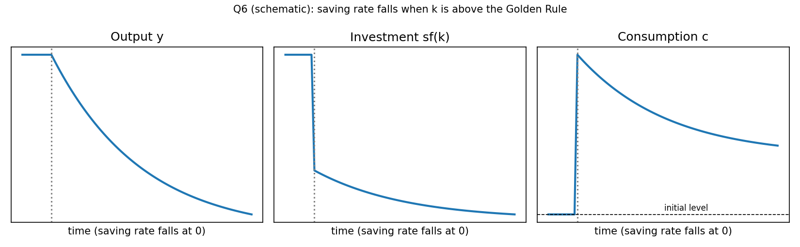
Schematic (illustrative parameters, not from the exam). Output and investment fall throughout. Consumption jumps up, declines, and settles above where it started.
- B. False. Consumption jumps up at once, so it does not fall at all.
- C. False. Right on direction at first, but too loose: consumption does not keep rising, it falls back after the jump (though it stays above its start).
- D. False. Gets the path right but the destination wrong. Starting above the golden rule, the new steady-state consumption is higher, not lower. It would be lower only if the economy started below the golden rule.
🗣️ In plain EnglishThe economy has too much capital. Saving less lets people consume more right away, and even after capital shrinks back they still end up consuming more than before.
Q7 — Constant returns to capital
AI-written answer, consistent with the tofes 0 layout (answer printed first).Outside the lecture notes (growth, Ch 8-9). Solved from the standard endogenous-growth setup.
Question. The endogenous growth model's assumption of constant returns to capital is more plausible if capital is defined to include:
- A. knowledge (human capital).
- B. factories and equipment.
- C. depreciation.
- D. technology.
Answer: A
The AK model is : no diminishing returns to capital. That is implausible for physical capital alone (more machines per worker eventually add less). If "capital" is defined broadly to include knowledge and human capital, there is no obvious reason for diminishing returns: ideas and skills can keep accumulating and spill over.
- B. False. Physical capital is exactly where diminishing returns are most believable (the Solow case).
- C. False. Depreciation is a flow that erodes capital, not a type of capital.
- D. False. In Solow, technology is the separate factor (exogenous). Option A is the wording that fits the broad-capital argument. A tempting trap, since "technology" sounds like knowledge.
🗣️ In plain EnglishMachines run into diminishing returns, but knowledge and skills keep building on each other. So the "capital doesn't hit diminishing returns" idea fits better if capital includes human capital.
Q8 — Golden-rule saving rate
AI-written answer, consistent with the tofes 0 layout (answer printed first).Outside the lecture notes (Solow, Ch 8-9 has no deck). Solved from the standard Solow model.
Question. In the steady state of the Solow model, with Cobb-Douglas production, the saving rate should be _______ the _______ share of the national income, so that golden-rule applies.
- A. equal to, capital.
- B. greater than, capital.
- C. lower than, capital.
- D. equal to, labor.
Answer: A
Golden rule: (with ). For Cobb-Douglas , . The steady state has . Substituting gives , so
- B and C. False. Saving above is dynamically inefficient (too much capital); below is too little. Only equality maximises steady-state consumption.
- D. False. The relevant share is the capital share . Labour's share is .
🗣️ In plain EnglishTo get maximum consumption in the long run, save the same fraction of income as the capital share of income.
Q9 — Solow vs endogenous growth
AI-written answer, consistent with the tofes 0 layout (answer printed first).Outside the lecture notes (growth, Ch 8-9). Solved from the standard models.
Question. Which of the following is a key difference between the Solow growth model and the endogenous growth theory (like the two-sector model)?
- A. The Solow model assumes technological progress is exogenous, while endogenous growth theory explains technological progress as a result of economic decisions.
- B. The Solow model predicts perpetual growth without technological progress, while endogenous growth theory predicts diminishing returns to capital.
- C. The Solow model assumes increasing returns to capital, while endogenous growth theory assumes diminishing returns to capital.
- D. The Solow model considers knowledge as the primary driver of growth, while endogenous growth theory ignores the role of knowledge.
Answer: A
In Solow, (the growth rate of efficiency) is exogenous: it is a given. Endogenous growth models (AK, the two-sector model with a research sector) make long-run growth the result of decisions such as how much to invest in knowledge and human capital.
- B. False, and backwards. Solow with no technological progress ends in a steady state with zero per-worker growth. It is endogenous growth (AK) that predicts perpetual growth, because it has no diminishing returns to (broad) capital.
- C. False, and backwards. Solow has diminishing returns to capital. Endogenous growth (AK) has constant returns.
- D. False, and backwards. Solow treats knowledge () as given, an outside force. Endogenous growth is the theory that puts knowledge at the centre.
🗣️ In plain EnglishIn Solow, technology falls from the sky. In endogenous growth, people choose to produce it.
Q10 — A demand shock
AI-written answer, consistent with the tofes 0 layout (answer printed first).
Question. Which of the following is an example of a demand shock that could shift the aggregate demand curve to the right?
- A. A sudden increase in consumer confidence
- B. An increase in oil prices
- C. A technological innovation that increases productivity
- D. A rise in nominal wages
Answer: A
Higher consumer confidence raises at every price level, shifting AD right (the IS curve shifts right, see Aggregate Demand Curve and Demand Shock).
- B. False. An oil price rise is a Supply Shock: it raises costs and shifts SRAS up/left.
- C. False. A productivity gain is a supply-side shock (it shifts SRAS/LRAS to the right).
- D. False. Higher nominal wages are a cost for firms, so they shift SRAS up/left. They are not an exogenous rise in spending.
🗣️ In plain EnglishA demand shock is a change in how much people want to spend. Feeling more confident makes them spend more. Oil, technology and wages hit the cost and supply side instead.
Q11 — Long-run equilibrium from point A
AI-written answer, consistent with the tofes 0 layout (answer printed first).The graph is not in the PDF; it is taken from the
.docxof the same paper.
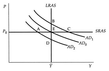
Question. In this graph, initially the economy is at point A. Where would the long-run equilibrium be (assuming no government intervention)?
- A. D
- B. C
- C. E
- D. B
Answer: A (point D)
Point A is where (the lowest curve) crosses the flat at , to the left of . So output is below natural, slack in the economy. With no intervention, the economy self-corrects: expected/actual prices fall, SRAS shifts down, and the economy slides down along until output returns to on the vertical LRAS. That point is D: natural output, a lower price level than . See Long-Run Aggregate Supply, Aggregate Demand Curve and Lec_06-AS-AD Model & Economic Fluctuations.
- B. (C) is on with output above . It is not on the same AD curve and not on LRAS.
- C. (E) is the original equilibrium on . Without a policy that shifts AD back from to , the economy does not return there. "No government intervention" rules out that rescue.
- D. (B) is on LRAS but at a higher price level, on . Reaching it needs AD to rise, not fall.
IntuitionLeft alone, a recession ends with deflation, not with a return to the old price level. The price level adjusts, not AD.
🗣️ In plain EnglishThe economy starts in a slump. If nobody steps in, prices fall until output is back to normal, ending at D, with lower prices than before.
Q12 — Two central banks and an oil shock
AI-written answer, consistent with the tofes 0 layout (answer printed first).
Question. Assume the AD-AS model with fixed prices in the short run. If Central Bank A cares only about restoring the price level to its original level and Central Bank B cares only about keeping output at its natural level at all times, then in response to an exogenous increase in the price of oil:
- A. Central Bank A should keep the quantity of money stable whereas Central Bank B should increase it.
- B. both Central Bank A and Central Bank B should increase the quantity of money.
- C. Central Bank A should increase the quantity of money whereas Central Bank B should keep it stable.
- D. both Central Bank A and Central Bank B should keep the quantity of money stable.
Answer: A
A higher oil price is an adverse Supply Shock: SRAS shifts up, so the price level rises and output falls below (Stagflation). Two responses:
-
Bank B (output only): shift AD right by raising , so output returns to at once. Cost: the price level stays higher (it accommodates the shock).
-
Bank A (price level only): do nothing. Left alone, slack pushes prices down over time, SRAS drifts back and the economy returns to at the original price level, so A's goal is met by keeping stable. Raising would move the price level further from the original.
-
B. False. Raising is wrong for Bank A: it pushes the price level up, away from its target.
-
C. False. Reversed: it asks A to be the one that accommodates.
-
D. False. Fine for A, but Bank B would be left with output stuck below for the long adjustment, which violates "at all times".
Reading of "restoring the price level"A bank that wanted to restore the price level immediately could also cut (shift AD left), at the cost of an even deeper recession. That choice is not among the options, so the only consistent reading is "keep stable and let prices adjust". See Stabilization Policy and Lec_06-AS-AD Model & Economic Fluctuations.
🗣️ In plain EnglishAfter an oil shock, a bank that wants full employment now must print money. A bank that only wants prices back to normal can just wait.
Q13 — Income at Y3 in the Keynesian cross
AI-written answer, consistent with the tofes 0 layout (answer printed first).The graph is not in the PDF; it is taken from the
.docxof the same paper.
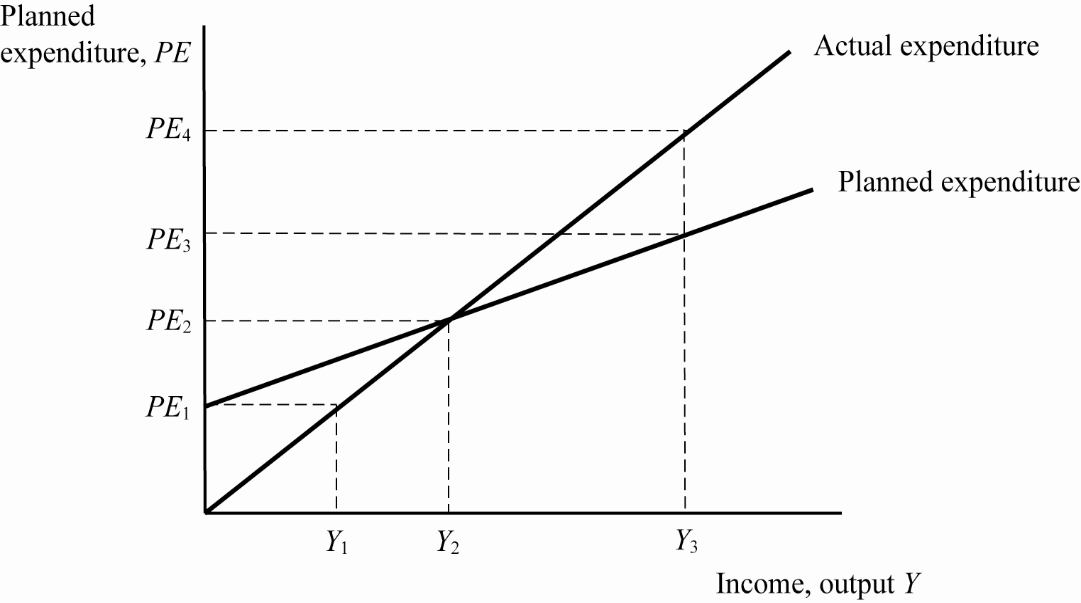
Question. Assume that income level is . What will happen?
- A. inventory will accumulate above the planned level, production rate would thus fall.
- B. inventory will accumulate above the planned level, production rate would thus rise.
- C. inventory will fall below the planned level, production rate would thus fall.
- D. inventory will fall below the planned level, production rate would thus rise.
Answer: A
At actual expenditure (output) is but planned expenditure is only . Firms produce more than they sell, so unplanned inventories pile up. Firms respond by cutting production, so falls from toward the equilibrium where . See Keynesian Cross and Inventory Adjustment.
- B. False. Inventories accumulate, but firms with unsold stock do not raise production.
- C and D. False. They have the gap the wrong way round. Inventories fall below plan at , where planned expenditure () exceeds output (and there firms raise production).
🗣️ In plain EnglishAt firms make more than people buy, so goods pile up unsold and firms slow production until it matches spending.
Q14 — Why the LM curve slopes up
AI-written answer, consistent with the tofes 0 layout (answer printed first).
Question. The LM curve slope can be explained as follows
- A. when income rises, people want to consume more, so they increase the demand for money and inflate the interest rate.
- B. when the interest rate falls, investment rise so the GDP level increases as well.
- C. when the interest rate rises people consume more and subsequently the GDP level rises
- D. when income rises, people want to consume more, so the supply of money rises and inflate the interest rate.
Answer: A
LM is the money market. With real balances fixed, higher income raises money demand (more transactions). To clear the market, the interest rate must rise to cut money demand back. That gives an upward-sloping LM. See LM Curve and Liquidity Preference.
- B. False. This describes the IS curve (lower raises and ), which slopes down.
- C. False. Higher reduces investment and spending. It is also IS logic.
- D. False. Money supply is set by the central bank ( fixed along LM). A rise in income does not raise it.
🗣️ In plain EnglishHigher income means people want more money to spend. With a fixed supply of money, the price of money (the interest rate) must rise.
Q15 — Tax cut vs spending multiplier
AI-written answer, consistent with the tofes 0 layout (answer printed first).
Question. In the IS-LM analysis, the increase in income resulting from a tax cut is usually ______ the increase in income resulting from an equal rise in government spending.
- A. less than
- B. greater than
- C. equal to
- D. sometimes less and sometimes greater than
Answer: A
In the Keynesian cross, the government-spending multiplier is and the tax-cut multiplier is . Since , the tax multiplier is smaller. A $1 spending rise adds $1 of demand directly, whereas a $1 tax cut adds only of it, because part is saved. The IS shift is therefore smaller for a tax cut, and so is the final rise in . See Fiscal Multiplier and Marginal Propensity to Consume.
- B. False. It would need , which is not possible.
- C. False. Equal only if .
- D. False. The ranking holds for any , so it is not situation-dependent.
🗣️ In plain EnglishGovernment spending is a direct injection. A tax cut is only partly spent, since some is saved. So spending gives a bigger boost.
Q16 — Steady-state capital per effective worker
AI-written answer, consistent with the tofes 0 layout (answer printed first).Outside the lecture notes (Solow, Ch 8-9 has no deck). Solved from the standard Solow model with technological progress.
Question. An economy follows the Solow growth model with technological progress. The production function per effective worker is . The saving rate is , depreciation , population growth , technological growth . What is the steady-state level of capital per effective worker, ?
- A. 4.63
- B. 3.92
- C. 4.07
- D. all other answers are wrong
Answer: A ()
In steady state, saving per effective worker covers depreciation plus dilution by and :
I checked the arithmetic numerically: .
- B (3.92) and C (4.07). False. Neither comes from the formula. For example, leaving out gives , which is not among the options either.
- D. False, since A is right.
🗣️ In plain EnglishCapital settles where new saving exactly makes up for wear and tear and the growing number of effective workers. Plugging in the numbers gives 4.63.
Q17 — Keeping the interest rate constant after a spending cut
AI-written answer, consistent with the tofes 0 layout (answer printed first).The graph is not in the PDF; it is taken from the
.docxof the same paper.
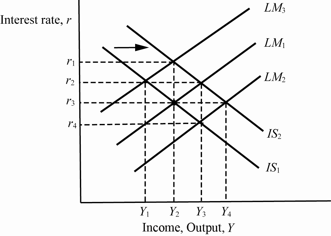
Question. Starting from equilibrium at interest rate , income , if there is a decrease in government spending, then in order to keep the interest rate constant at , the Federal Reserve should _____ the money supply shifting to _____.
- A. decrease; LM3
- B. increase; LM2
- C. decrease; LM2
- D. increase; LM3
Answer: A (decrease; )
The starting equilibrium is crossing at . A cut in shifts the IS curve left, to . If the Fed did nothing, the new equilibrium ( with ) would be at : lower income and a lower rate. To hold at , the LM curve must move up/left, which means a decrease in (see Fiscal Multiplier and Monetary-Fiscal Policy Interaction). meets at , and is the curve through . Income falls even more, to .
- B. False. lies below/right of (an increase in ). It meets at (lower than ), the opposite of what is wanted. It would also cushion output rather than hold the rate.
- C. False. Right direction (decrease) but is the curve for an increase in .
- D. False. Raising shifts LM down/right, not to (the up/left curve). The word and the curve contradict each other, and an increase would let fall to .
IntuitionLower spending would pull the interest rate down. To stop the rate falling, the central bank must tighten, at the cost of an even bigger fall in output.
🗣️ In plain EnglishLess government spending would normally lower interest rates. To hold the rate steady the Fed has to shrink the money supply, which makes the fall in income bigger.
Q18 — What happens in the long run when prices adjust
AI-written answer, consistent with the tofes 0 layout (answer printed first).
Question. In the IS-LM model, what happens in the long run when the price level adjusts?
- A. The LM curve shifts due to changing real money balances
- B. The IS curve shifts leftward
- C. The economy remains at the short-run equilibrium
- D. The IS and LM curves move together to keep output constant
Answer: A
The price level enters through . If , prices fall, real balances rise and LM shifts right (if , prices rise and LM shifts left) until . IS does not depend on . See Lec_08-Aggregate Demand II & Applying the IS-LM Model and Money Neutrality (LR).
- B. False. does not appear in the IS curve, so it does not shift when prices adjust. IS shifts only with , , or confidence.
- C. False. The short-run equilibrium generally has , and the pressure on continues until . It is not stable in the long run unless it already sits at .
- D. False. Only LM moves, and it moves toward , not "together with" IS to hold output fixed.
🗣️ In plain EnglishWhen prices change, the real value of money changes, so the LM curve moves until output is back to normal. The IS curve stays put.
Q19 — Solving an IS-LM system
AI-written answer, consistent with the tofes 0 layout (answer printed first).
Question. Consider the following IS-LM model: , , , , , , . What is the equilibrium level of income and the equilibrium interest rate?
- A. ,
- B. ,
- C. ,
- D. ,
Answer: A
IS. :
LM. Real balances , and money market clears when :
Solve. , so . See IS-LM Equilibrium.
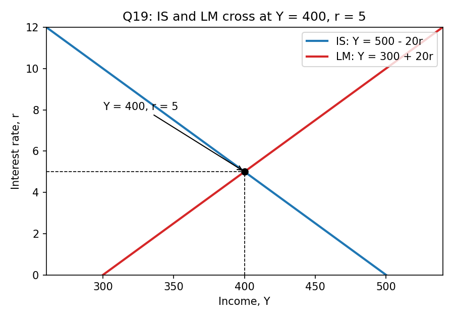
IS slopes down, LM slopes up. They cross at , .
- B (, ). LM gives , not 520. Fails.
- C (, ). LM gives and IS gives . Fails both.
- D (, ). LM gives and IS gives . Fails both.
Check shortcutTest each option in both equations. Only A passes both.
🗣️ In plain EnglishWrite the IS and LM lines and see where they meet: income of 400 and an interest rate of 5%.
Q20 — Interest rate under perfect capital mobility
AI-written answer, consistent with the tofes 0 layout (answer printed first).
Question. In the Mundell-Fleming model, assuming perfect capital mobility, the domestic interest rate is determined by:
- A. The world interest rate
- B. The domestic central bank
- C. The level of government spending
- D. The money demand function
Answer: A
Perfect Capital Mobility in a small open economy means arbitrage forces . Any gap would trigger immediate capital flows until the rates equalise. See Mundell-Fleming Model and Lec_09-The Open Economy Revisited & Mundell-Fleming Model.
- B. False. The central bank can move but cannot change away from (under floating rates the exchange rate or income adjusts instead).
- C. False. Fiscal policy shifts IS*, not the interest rate.
- D. False. Money demand determines income (along LM*), not the interest rate, which is pinned at .
🗣️ In plain EnglishMoney flows to wherever interest is highest, so a small open economy's rate is stuck at the world rate.
Q21 — Money expansion with a floating exchange rate
AI-written answer, consistent with the tofes 0 layout (answer printed first).
Question. If the money supply increases in a small open economy with a floating exchange rate, what happens to the exchange rate and output?
- A. The exchange rate depreciates, and output increases
- B. The exchange rate depreciates, and output remains unchanged
- C. The exchange rate appreciates, and output decreases
- D. The exchange rate remains constant, and output decreases
Answer: A
Higher shifts LM* to the right. With fixed, the exchange rate must fall (depreciate) to restore equilibrium, which raises net exports, and output rises. See Floating Exchange Rate and LM* Curve.
- B. False. Output is not unchanged. That is the result for a fiscal expansion under floating rates (the exchange rate absorbs it).
- C. False. A larger money supply lowers the domestic rate, which pushes capital out and depreciates the currency.
- D. False. A floating rate moves, and output does not fall.
🗣️ In plain EnglishMore money makes the currency weaker, which boosts exports, so output rises.
Q22 — Fiscal expansion under a fixed exchange rate
AI-written answer, consistent with the tofes 0 layout (answer printed first).
Question. Suppose a country has a fixed exchange rate and wishes to maintain it while increasing government spending. What must the central bank do?
- A. Increase the money supply to prevent appreciation
- B. Reduce the money supply to maintain the exchange rate
- C. Do nothing, as fiscal policy has no effect under fixed exchange rates
- D. Allow the exchange rate to float freely
Answer: A
More shifts IS* right. That pushes the exchange rate up (appreciation pressure). To hold the peg the central bank must sell domestic currency, which raises and shifts LM* right until the exchange rate is back at the peg. Output rises, so fiscal policy is powerful under fixed rates. See Fixed Exchange Rate.
- B. False. Cutting would push the currency further up, away from the peg.
- C. False. The reverse: fiscal policy is effective under fixed rates (it is monetary policy that is powerless).
- D. False. Floating abandons the stated goal of maintaining the rate.
🗣️ In plain EnglishMore government spending pushes the currency up. To keep the peg, the central bank must create money, which adds to the boost in output.
Q23 — The Phillips curve trade-off
AI-written answer, consistent with the tofes 0 layout (answer printed first).
Question. The Phillips curve suggests that in the short run, policymakers face a tradeoff between:
- A. Inflation and unemployment
- B. Inflation and interest rates
- C. The budget deficit and GDP
- D. Government spending and net exports
Answer: A
The Phillips Curve links inflation and unemployment: lower unemployment comes with higher inflation in the short run. See Lec_14-Aggregate Supply & the Phillips Curve.
- B, C, D. False. None of these pairs is what the curve describes (B is the Fisher relationship, C and D are IS-side relationships).
🗣️ In plain EnglishIn the short run you can get lower unemployment, but only at the price of higher inflation.
Q24 — Higher inflation expectations
AI-written answer, consistent with the tofes 0 layout (answer printed first).
Question. If inflation expectations increase, what happens to the short-run Phillips curve?
- A. It shifts upward
- B. It shifts downward
- C. It becomes vertical
- D. It remains unchanged
Answer: A
. A higher adds to inflation at every level of unemployment, so the short-run curve shifts up. See Adaptive Expectations and Inflation Inertia.
- B. False. Lower expectations would shift it down.
- C. False. The curve is vertical only in the long run (at ), not because expectations rose.
- D. False. Expected inflation is the intercept of the curve, so changing it moves the curve.
🗣️ In plain EnglishIf people expect more inflation, wages and prices get set higher, so inflation is higher at every unemployment rate.
Q25 — Phillips curve arithmetic
AI-written answer, consistent with the tofes 0 layout (answer printed first).
Question. Suppose the Phillips curve is , where is expected inflation, is unemployment, is the natural rate of unemployment (5%), and is a supply shock. If expected inflation is 3%, actual unemployment is 7%, and there is no supply shock, what is actual inflation?
- A. 2%
- B. 3%
- C. 4%
- D. 5%
Answer: A
Unemployment is 2 points above natural, which pulls inflation 1 point below expectations. See Natural Rate of Unemployment and Cyclical Unemployment.
- B (3%). Would hold only if . Here there is slack, so inflation is below expectations.
- C (4%). Sign error: adds instead of subtracting it.
- D (5%). Adds the full gap of 2 and ignores the 0.5 slope.
🗣️ In plain EnglishUnemployment is above normal, which holds inflation below what people expected. Expected 3%, minus 1 point from the slack, gives 2%.
Recap table
| Q | Topic | Answer | One line |
|---|---|---|---|
| 1 | Real wage | A | , so productivity raises it |
| 2 | Investment demand shock | A | fixed, so only rises |
| 3 | Velocity | A | , so |
| 4 | Announced money growth | A | Fisher effect cuts money demand, so jumps by more than 3% |
| 5 | Classical dichotomy | A | falls, real variables unchanged |
| 6 | Above golden rule, falls | A | jumps, falls back, ends higher |
| 7 | AK constant returns | A | Plausible if capital includes human capital |
| 8 | Golden rule saving | A | (capital share) |
| 9 | Solow vs endogenous | A | Exogenous vs endogenous technology |
| 10 | Demand shock | A | Consumer confidence |
| 11 | Long run from A | A | Point D: natural output, lower |
| 12 | Oil shock, two banks | A | A waits, B raises |
| 13 | Keynesian cross at | A | Inventories pile up, production falls |
| 14 | LM slope | A | Income raises money demand, so rises |
| 15 | Tax vs spending | A | |
| 16 | A | ||
| 17 | Hold after cut | A | Decrease , to |
| 18 | Long-run price adjustment | A | LM shifts via |
| 19 | IS-LM numbers | A | , |
| 20 | Perfect capital mobility | A | |
| 21 | up, floating | A | Depreciates, rises |
| 22 | up, fixed rate | A | Increase to defend the peg |
| 23 | Phillips trade-off | A | Inflation vs unemployment |
| 24 | Expectations up | A | SRPC shifts up |
| 25 | Phillips arithmetic | A |
Related notes
Macro-Economics II · Lec_03-Classical Theory & National Income · Lec_05-Inflation · Lec_06-AS-AD Model & Economic Fluctuations · Lec_07-Aggregate Demand I & the IS-LM Model · Lec_08-Aggregate Demand II & Applying the IS-LM Model · Lec_09-The Open Economy Revisited & Mundell-Fleming Model · Lec_14-Aggregate Supply & the Phillips Curve