
Macro II Moed B 2021 — Worked Solutions
- #macro-economics-ii
- #past-paper
- #worked-solution
- #multiple-choice
- #solow
- #as-ad
- #is-lm
- #mundell-fleming
- #phillips-curve
Macro II Moed B 2021 — Worked Solutions
Part of: Macro-Economics II Moed B, 23 August 2021 — Macroeconomics II (3058), Dr. Alon Cohen. 25 multiple-choice questions, 4% each, open books, 2.5 hours. Builds on: Lec_03-Classical Theory & National Income · Lec_04-The Monetary System · Lec_05-Inflation · Lec_06-AS-AD Model & Economic Fluctuations · Lec_07-Aggregate Demand I & the IS-LM Model · Lec_08-Aggregate Demand II & Applying the IS-LM Model · Lec_09-The Open Economy Revisited & Mundell-Fleming Model · Lec_14-Aggregate Supply & the Phillips Curve
ALL 25 questions are AI-solved. There is no official key.This is a tofes 0 paper (master version, correct answer printed first as A) and no key is in the source folder. I solved each question independently first, then compared with option A. I got A on all 25, but see the two flags below. Not official. Check before relying on it.
- Q4 (Solow, persistent growth): in the no-technology Solow model the textbook answer is "no" (option C). A is only right if you read the question as including technological progress. Flagged at the question.
- Q9 (Okun's Law): plugging the figures in literally gives a 4 point rise, which is not an option. A (2.5) works only under the reading explained at the question.
- Q1-Q6 are Solow growth (Ch 8-9), which has no lecture deck in this course. Solved from the standard Solow model.
What this paper tests
The paper in one paragraphThe first 6 questions are Solow growth, then the usual short-run machinery.
- Solow (Q1-Q6): steady state with unemployment, saving rate, golden rule, growth in the steady state.
- AS-AD (Q7-Q9, Q16, Q25): fixed-price AD-AS, Okun's Law, long-run monetary neutrality.
- Keynesian cross, IS-LM (Q10-Q15, Q17): multiplier, liquidity preference, fixed M vs fixed r, balanced-budget change.
- Mundell-Fleming (Q18-Q21): capital mobility, floating-rate policy, fixed-rate quota.
- Inflation and Phillips curve (Q22-Q24): inertia, demand-pull vs cost-push, the unemployment-inflation trade-off.
The recurring trick: floating-rate M-F has a vertical LM*, so fiscal and trade shocks only move the exchange rate (Q19, Q20).
Q1 — Output per worker with unemployment (Solow)
AI-written answer, not official. Check before relying on it.Outside the lecture notes (Solow, Ch 8-9 has no deck). Consistent with the tofes 0 layout (answer printed first).
Question. Consider the Solow model with no technological progress and the production function , where is output, is the labor force, is the unemployment rate and is the capital. Depreciation is 10%, labor force growth is 2.5% and the saving rate is 25%. By how much will output per worker fall, in the steady state, if unemployment marginally rises?
- A.
- B.
- C.
- D.
Answer: A (AI-solved)
Only the employed produce, so effective labor is . Per worker (of the labor force), with :
Steady state: investment per worker equals break-even investment, .
So : a marginal rise in lowers steady-state output per worker by 2 per unit.
- B () and D (). Would need or , i.e. a saving rate of about 12.5% or 6%.
- C (). Does not come out of the algebra. Holding fixed (ignoring that also falls with ) would give a different, smaller number, so C is a distractor.
IntuitionUnemployment hits twice: fewer workers per unit of capital-labor input directly, and a smaller labor input means less capital is sustained ( falls with ). Both effects are inside the factor .
🗣️ In plain EnglishHigher unemployment shrinks the part of the labor force that actually works. In the steady state that works out as , so each extra bit of unemployment costs 2 units of output per worker.
Q2 — Saving more: guaranteed short-run gains?
AI-written answer, not official. Check before relying on it.Outside the lecture notes (Solow). Consistent with the tofes 0 layout (answer printed first).
Question. Assume the Solow model with no population growth or technological progress. A steady-state economy decides to devote a larger share of its output to investment. Short run gains for living standards (consumption) and productivity (output per worker) are guaranteed. True or False?
- A. False. In the short run living standard will fall and productivity will rise.
- B. False. In the short run living standard will fall and productivity will fall.
- C. False. In the short run living standard will rise and productivity will fall.
- D. True.
Answer: A (AI-solved)
A higher saving rate means consumption drops at once: output has not changed yet, but a bigger share goes to investment. Investment now exceeds break-even investment, so rises and so does output per worker , gradually, toward the new steady state. Consumption then recovers over time (and ends higher only if the economy was below the golden rule).
- B. Productivity does not fall: more capital per worker means more output per worker.
- C. Backwards. Consumption cannot rise on impact when the saving share rises.
- D. "Guaranteed" is false because consumption falls first.
🗣️ In plain EnglishSaving more means less to spend today, so living standards dip first. The extra investment builds capital, so output per worker climbs over time.
Q3 — Higher saving rate in the Solow model
AI-written answer, not official. Check before relying on it.Outside the lecture notes (Solow). Consistent with the tofes 0 layout (answer printed first).
Question. In the Solow growth model, with a given production function, depreciation rate, no technological change, and no population growth, a higher saving rate produces a:
- A. higher steady-state level of output per worker.
- B. higher steady-state growth rate of total output.
- C. higher steady-state growth rate of output per worker.
- D. higher MPK in the new steady state.
Answer: A (AI-solved)
Steady state: . A higher shifts the investment curve up, so and are higher. This is a level effect.
- B. With no population growth or technology, steady-state growth of total output is zero, whatever is. It is only temporarily positive during the transition.
- C. Growth of output per worker is also zero in the steady state. changes the level, not the long-run growth rate.
- D. More capital per worker means a lower marginal product of capital (diminishing returns). In the steady state falls when rises.
🗣️ In plain EnglishSaving more gives you a higher level of output per worker in the long run, but not faster growth forever. Growth stops once you reach the new steady state.
Q4 — Persistent growth in living standards inside a steady state
AI-written answer, not official. Check before relying on it. FLAGGED FOR ALFIE.Outside the lecture notes (Solow). My independent solve disagrees with A under the strict no-technology reading (I would pick C). I keep A as the likely official answer: it is the tofes 0 first option and it is correct once technological progress is allowed.
Question. According to the Solow model: is a persistent growth in the standards of living within a steady-state economy possible?
- A. Yes, provided that capital stock grows faster than the labor force
- B. Yes, provided that capital stock grows slower than the labor force
- C. No, because capital stock always grows as fast as the labor force
- D. No, because capital stock grows slower than the labor force
Answer: A (AI-solved, likely official)
Living standards (, output per worker) can only keep growing if capital grows faster than labor. In the model with technological progress at rate , the steady state has capital per effective worker constant, so grows at while grows at . Capital therefore grows faster than the labor force, and output per worker grows at . So "yes, provided capital grows faster than labor" is the condition, and technological progress is what delivers it.
- B. If capital grew slower than labor, capital per worker would fall, so living standards would fall.
- C. This is the correct statement for the basic Solow model (no technology): in the steady state is constant, so grows at exactly , the same as , and there is no per-worker growth. That is my independent answer if the question means no technological change. The question does not say "no technological progress" (Q1 and Q3 do), which is why A is the better fit.
- D. Same as B: shrinking capital per worker cannot raise living standards.
🗣️ In plain EnglishLiving standards only keep rising if each worker gets more and more capital, meaning capital must grow faster than the labor force. In the Solow model that only happens with technological progress.
Q5 — Is the return to capital fixed with technological progress?
AI-written answer, not official. Check before relying on it.Outside the lecture notes (Solow). Consistent with the tofes 0 layout (answer printed first).
Question. Under the Solow model with technological progress, the return to capital is fixed. True or false?
- A. True, because capital per efficient worker is fixed in the steady state.
- B. True, because capital per efficient worker has constant returns, whenever the production function has constant returns
- C. True, because the share of capital in national income is fixed
- D. False, because capital per efficient worker has diminishing returns whenever the production function has constant returns
Answer: A (AI-solved)
With technological progress the steady state has capital per efficient worker constant. The return to capital is , a function of only. If is fixed, so is the return to capital, even though keeps growing.
- B. False reasoning: capital per efficient worker has diminishing returns (that is why falls as rises), not constant returns.
- C. The capital share is constant for Cobb-Douglas, but that is a property of a particular function, not why the return is fixed in general.
- D. The reasoning is true (diminishing returns to ) but the verdict "False" is wrong: with fixed in the steady state, the return is fixed.
🗣️ In plain EnglishMeasured per efficient worker, the amount of capital stays put in the steady state. Since the return to capital depends only on that amount, it stays fixed too.
Q6 — Freedonia: what tax advice?
AI-written answer, not official. Check before relying on it.Outside the lecture notes (Solow). Consistent with the tofes 0 layout (answer printed first).
Question. In Freedonia the return to capital is 15%, depreciation rate is 7% and output growth rate is 4%. What would you advise that country to do?
- A. Cut taxes on capital gains
- B. Replace consumption tax with income tax
- C. Increase taxes on capital gains
- D. Narrow tax benefits for retirement saving accounts
Answer: A (AI-solved)
Golden-rule test: the golden-rule capital stock has (the net return equals output growth). Here , which is above . A high net return to capital means capital is scarce: the economy is below the golden rule and should save and invest more. Cutting capital-gains taxes raises the after-tax return to saving and encourages it.
- B. Income tax taxes the return to saving (double taxation), so it discourages saving. Replacing a consumption tax with an income tax pushes the wrong way.
- C. Taxing capital gains more discourages saving: wrong direction.
- D. Narrowing retirement-account benefits removes a saving incentive: wrong direction.
🗣️ In plain EnglishA net return of 8% against 4% growth says the country has too little capital. It should encourage saving, for example by cutting taxes on capital gains.
Q7 — Fed stabilization with fixed prices
Question. Assume the AD-AS model with fixed price level in the short run. If the Fed is interested in maintaining price level and employment rate stable, at all times, which shock will it be able to cope with better?
- A. A shock to the demand
- B. A shock to the supply
- C. The Fed can never maintain stable prices and employment, in either type of shock
- D. Either a shock to the demand or to the supply can be addressed by the Fed such that prices and employment remain stable
AI-written answer, not official. Check before relying on it.Consistent with the tofes 0 layout (answer printed first). See Lec_06-AS-AD Model & Economic Fluctuations.
Answer: A (AI-solved)
A Demand Shock moves AD. The Fed can move AD back with Stabilization Policy (change ), so output and price both return to where they were. Both goals are met at once.
A Supply Shock shifts SRAS. The Fed can only choose where on the new AS curve to land: offset the shock with AD and it keeps output stable but prices move; hold prices and output moves. It faces a trade-off.
- B. Reversed: supply shocks create the trade-off.
- C. Too strong: demand shocks can be fully offset.
- D. Only demand shocks can be fully offset.
🗣️ In plain EnglishA demand shock can be cancelled by moving demand back. A supply shock forces a choice between stable prices and stable output.
Q8 — Is long-run money neutrality in the AD-AS model?
Question. Monetary neutrality, the irrelevance of the money supply in determining values of real variables, is generally thought to be a property of the economy just in the long run. Does the AD-AS model support that argument?
- A. Yes. Prices change proportionally to any change in the money supply, offsetting in the long-run any short-run effect over real variables
- B. Yes. Stabilizing policy always restores output and unemployment to its normal rates in the long-run
- C. No. A change in money supply does affect unemployment and output both in the short-run and in the long-run
- D. No. A change in money supply does not affect unemployment and output both in the short-run and in the long-run
AI-written answer, not official. Check before relying on it.Consistent with the tofes 0 layout (answer printed first).
Answer: A (AI-solved)
In the short run prices are sticky, so a change in shifts AD and moves and . Over time prices adjust, SRAS shifts, and the economy returns to at a price level that has changed in proportion to . Real variables are back where they started. This is Money Neutrality (LR). Q25 draws exactly this.
- B. Right outcome, wrong cause: the long-run return to comes from price adjustment, not from stabilizing policy. It would happen with no policy at all.
- C. Wrong in the long run: real variables are unaffected.
- D. Wrong in the short run: with sticky prices real variables do move.
🗣️ In plain EnglishPrinting money moves output only until prices catch up. In the long run prices rise in proportion, and real things are back to normal.
Q9 — Money supply cut and unemployment (Okun's Law)
AI-written answer, not official. Check before relying on it. FLAGGED FOR ALFIE.Literal substitution gives a rise of 4, which is not an option. A (rise by 2.5) is reached under the reading below. Consistent with the tofes 0 layout (answer printed first).
Question. Assume the AD-AS model with fixed price level, , and the economy is in a benchmark long-run equilibrium. The AD curve is given by where is some constant and is money supply. If the central bank decreases money supply by 5%, what will happen to unemployment rate (recall Okun's Law: )?
- A. Rise by 2.5%
- B. Fall by 2.5%
- C. Fall by 5%
- D. Fall by 4%
Answer: A (AI-solved)
Step 1. With fixed, , so a 5% fall in lowers by 5%.
Step 2. Output falls, so unemployment rises. That already rules out B, C and D (all falls).
Step 3, size. Okun's Law says output growth is the 3% trend minus . The economy starts in long-run equilibrium, so before the shock it is at its benchmark level. The AD cut puts output 5% below the benchmark: the 5% fall is the deviation from trend, so points. (Equivalently: trend growth of and a shock of gives , and .)
Check of the literal readingSubstituting straight into gives (a rise of 4). That is not offered, and D says "fall by 4". So the only consistent option is A, which needs the "5% below benchmark" reading above.
🗣️ In plain EnglishLess money means output drops 5%, which pushes unemployment up. By Okun's Law each 2% of lost output is about 1 point of unemployment, so roughly 2.5 points.
Q10 — Keynesian cross multiplier
Question. In the Keynesian-cross model with fixed interest rate, if the MPC equals 0.8, then a $1 billion increase in government spending, with no tax raise, spending increases planned expenditures by ______ and increases the equilibrium level of income by ______.
- A. $1 billion; $5 billion
- B. $1 billion; $1 billion
- C. $0.8 billion; $1 billion
- D. $0.8 billion; $5 billion
AI-written answer, not official. Check before relying on it.Consistent with the tofes 0 layout (answer printed first).
Answer: A (AI-solved)
Planned expenditure . The direct effect of is exactly $1 billion on . That extra spending becomes income, which raises consumption by income, and so on. The Fiscal Multiplier is
- B. Ignores the induced consumption: no multiplier.
- C and D. Planned expenditure rises by the full $1 billion from itself; is the first-round consumption response, which comes only after income rises.
🗣️ In plain EnglishThe government spends $1bn, so spending rises by $1bn straight away. That gets re-spent over and over, and total income ends up $5bn higher (the multiplier).
Q11 — Liquidity preference and the real money supply
Question. The theory of liquidity preference implies that, other things being equal, an increase in the real money supply will
- A. lower the interest rate
- B. raise the interest rate
- C. have no effect on the interest rate
- D. first lower and then raise the interest rate
AI-written answer, not official. Check before relying on it.Consistent with the tofes 0 layout (answer printed first).
Answer: A (AI-solved)
In Liquidity Preference, the interest rate adjusts so that money demand equals the (fixed) real money supply. More real money means people hold more than they want, so they buy bonds, bond prices rise and the interest rate falls until they are happy to hold the extra money.
- B. Opposite sign.
- C. True only in the long run in the classical model, not in liquidity preference with fixed income.
- D. There is no reversal: the rate falls to the new equilibrium and stays there.
🗣️ In plain EnglishMore money in the economy means people try to lend it out, so the interest rate falls.
Q12 — Money market arithmetic
Question. Assume that the money demand function is , where is the interest rate in percent. The money supply is 2,000 and the price level is 2. If the price level is fixed and the supply of money is raised to 2,800, then the equilibrium interest rate will
- A. drop by 2 percent
- B. drop by 4 percent
- C. drop by 1 percent
- D. remain unchanged
AI-written answer, not official. Check before relying on it.Consistent with the tofes 0 layout (answer printed first).
Answer: A (AI-solved)
Equilibrium: .
- Before: , so .
- After: , so .
The rate falls by 2 percentage points.
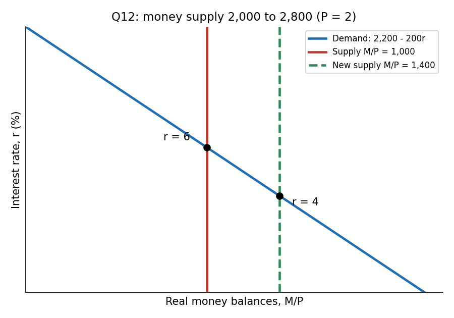
The supply line moves right from 1,000 to 1,400 along the downward demand curve, so goes from 6 to 4.
- B. A fall of 4 points (to ) needs . It is the trap of forgetting to divide the new by (or of the wrong direction of the shift).
- C. A fall of 1 point needs , i.e. .
- D. Wrong: with fixed, more money lowers (Q11).
🗣️ In plain EnglishDivide money by the price level (real balances go from 1,000 to 1,400) and solve . The interest rate falls from 6 to 4.
Q13 — How the goods and money markets connect
Question. According to the IS-LM model, how are the market for goods and services and the money market connected?
- A. Equilibrium in the money market determines the interest rate which affects investment and equilibrium in the market for goods and services; the latter, in turn determines income level which affects the demand for money and equilibrium in the money market
- B. Equilibrium in the money market determines income level which affects consumption and equilibrium in the market for goods and services; the latter, in turn determines interest rate which affects the equilibrium in the money market
- C. The market of goods and services determines income level and the money market determines interest rate, and the two are not connected
- D. Money market determines the interest rate, independently of the market for goods and services; the latter determines income level given the interest rate, which has no impact over the money market
AI-written answer, not official. Check before relying on it.Consistent with the tofes 0 layout (answer printed first).
Answer: A (AI-solved)
Two-way link. Interest rate feeds goods-market demand through investment (the IS curve). Income feeds the money market through money demand (the LM curve). Only the simultaneous solution gives . See IS-LM Equilibrium.
- B. Reverses the roles: the money market (with given) determines , and affects investment, not consumption through income.
- C. The markets are connected by and .
- D. Denies that income affects money demand, but it does: rises with .
🗣️ In plain EnglishThe interest rate drives investment, which drives income, and income drives money demand, which in turn sets the interest rate. Everything depends on everything else.
Q14 — Government spending rises in IS-LM
Question. In the IS-LM model when government spending rises, in short-run equilibrium, in the usual case the interest rate ______ and output ______.
- A. rises; rises
- B. rises; falls
- C. falls; rises
- D. falls; falls
AI-written answer, not official. Check before relying on it.Consistent with the tofes 0 layout (answer printed first).
Answer: A (AI-solved)
Higher shifts IS right. With LM unchanged (upward sloping), the new intersection has higher and higher . The higher partly Crowding Out investment, so rises by less than the Keynesian-cross multiplier suggests.
- B. does not fall: IS moves right, so output increases (just by less than the cross).
- C and D. cannot fall: the rightward IS move along an upward LM raises .
🗣️ In plain EnglishMore government spending boosts output, and it also pushes interest rates up, which slightly dampens private investment.
Q15 — Fixed money supply or fixed interest rate?
Question. The central bank can either keep money supply fixed or interest rate fixed. In which case will a stabilizing policy be more effective (in terms of minimizing changes to output level) as a response to adverse shock to demand in the IS-LM model?
- A. Fixed money supply is more effective against shocks to the demand for goods and services; fixed interest rate is more effective against shocks to the demand for money
- B. Fixed money supply is more effective against shocks to the demand for money; fixed interest rate is more effective against shocks to the demand for goods and services
- C. Fixed money supply is more effective against shocks to the demand for money as well as shocks to the demand for goods and services
- D. Fixed interest rate is more effective against shocks to the demand for money as well as shocks to the demand for goods and services
AI-written answer, not official. Check before relying on it.Consistent with the tofes 0 layout (answer printed first).
Answer: A (AI-solved)
This is the standard Poole result. Fixing leaves LM upward sloping, which cushions an IS shock: when IS moves, moves and partly offsets the output change. Fixing makes LM horizontal, so an IS shock moves fully.
For a money-demand (LM) shock, the logic reverses. If is fixed, the LM shifts and swings. If the central bank fixes it supplies whatever money is demanded, so LM does not move and is stable.
- B. Exactly reversed.
- C. Fixed is worse for LM shocks.
- D. Fixed is worse for IS shocks (no interest-rate cushion).
🗣️ In plain EnglishIf the shock hits spending, keep money fixed and let rates absorb some of it. If it hits money demand, keep the interest rate fixed so output isn't disturbed.
Q16 — LM shift and the AD curve (figure)
Question. Address the following figure (interest rate against income ; one IS curve and three LM curves (, ) above (, ) above (, )). Assume that the LM curve has shifted from to . What happens to the AD curve?
- A. If and this represents a movement along the AD curve; If and this represents a leftward shift of AD
- B. If and this represents a movement along the AD curve; If and this represents a rightward shift of AD
- C. If and this represents a leftward shift of the AD curve; If and this represents movement along AD
- D. In either case this represents a leftward shift of the AD curve
AI-written answer, not official. Check before relying on it.Consistent with the tofes 0 layout (answer printed first). I read the figure image: is the top line, so the shift is a leftward (upward) move of LM.
Answer: A (AI-solved)
The LM curve depends on real balances . A leftward LM shift means fell. Two ways:
- rises, fixed (): this is the price level changing, and the AD curve already plots against . So it is a movement along AD (to a higher and lower ).
- falls, fixed (): at the same , output is now lower. That is a change in a non-price variable, so AD shifts left.
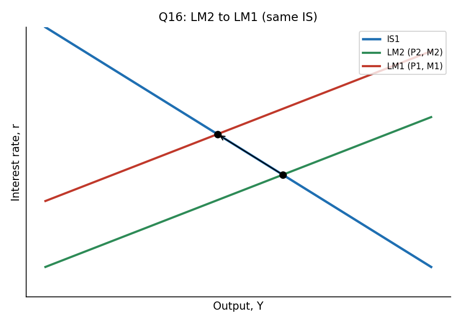
Same IS, LM moves up and left from to : the cause (price vs money) decides whether it is movement along AD or a shift.
- B. Right on the first case, but a money cut shifts AD left, not right.
- C. Reverses both cases.
- D. Wrong on the price case: a price change is a movement along AD.
🗣️ In plain EnglishIf prices push LM left, you're just sliding along the AD curve. If less money does it, the whole AD curve moves left.
Q17 — Balanced-budget increase in G and T
Question. According to the IS-LM model, when the government increases taxes and government purchases by equal amounts:
- A. income and the interest rate rise, whereas consumption and investment fall
- B. income, the interest rate, consumption, and investment are unchanged
- C. income and the interest rate fall, whereas consumption and interest rise
- D. income, the interest rate, consumption, and investment all rise
AI-written answer, not official. Check before relying on it.Consistent with the tofes 0 layout (answer printed first).
Answer: A (AI-solved)
Taxes up by . In the Keynesian cross this is the balanced-budget multiplier of 1: IS shifts right by . With LM upward sloping, rises, so rises by less than . Then:
-
Investment falls because rose (Crowding Out).
-
Consumption : disposable income changes by , so consumption falls.
-
B. IS does move, so and rise.
-
C. and do not fall; "consumption and interest rise" is also internally inconsistent (it means investment).
-
D. Consumption and investment cannot both rise: disposable income falls and rises.
🗣️ In plain EnglishGovernment spends more and taxes the same amount. Income and interest rates go up, but households are left with less take-home pay and firms invest less, so consumption and investment both fall.
Q18 — Small open economy, perfect capital mobility
Question. In a small open economy with perfect capital mobility, if the domestic interest rate were to rise above the world interest rate, then ______ would drive the domestic interest rate back to the level of the world interest rate
- A. capital inflow
- B. capital outflow
- C. the central bank
- D. a decline in domestic saving
AI-written answer, not official. Check before relying on it.Consistent with the tofes 0 layout (answer printed first).
Answer: A (AI-solved)
If , foreign savers rush to buy domestic assets. Capital inflow raises the supply of loanable funds at home and pushes down until . See Capital Mobility and Mundell-Fleming Model.
- B. Outflow happens when .
- C. The central bank is not needed: arbitrage alone does it.
- D. A fall in saving would raise , not lower it.
🗣️ In plain EnglishA high domestic rate attracts foreign money, which pushes the rate back down to the world rate.
Q19 — Cutting output under floating rates
Question. In a small open economy with a floating exchange rate, an effective policy to decrease equilibrium output is to:
- A. decrease the money supply
- B. increase the money supply
- C. decrease taxes
- D. decrease government spending
AI-written answer, not official. Check before relying on it.Consistent with the tofes 0 layout (answer printed first).
Answer: A (AI-solved)
Under floating rates is pinned down by , which is vertical: . Only (or money demand) moves it. A cut in shifts left, lowering (and raising the exchange rate). See LM* Curve and Floating Exchange Rate.
- B. Raises .
- C and D. Fiscal policy shifts , but the exchange rate adjusts and crowds out net exports one-for-one, so does not change.
🗣️ In plain EnglishUnder floating rates only monetary policy moves output. Fiscal changes get fully offset by the exchange rate.
Q20 — Taste for imports under floating rates (figure)
Question. Address the following figure (exchange rate against income ; vertical through A with to its left and to its right; through A, above it, below it). A small open economy with a floating exchange rate is initially in equilibrium at A with , . Holding all else constant, if domestic consumers develop greater preferences for imported goods, then the _____ curve will shift to _____.
- A. ;
- B. ;
- C. ;
- D. ;
AI-written answer, not official. Check before relying on it.Consistent with the tofes 0 layout (answer printed first). I viewed the figure: is the lowest (leftmost) IS line and the highest.
Answer: A (AI-solved)
A taste for imports lowers net exports at every exchange rate, so planned expenditure falls and shifts left/down, from to . does not depend on the trade balance, so it stays put. Output stays at the level and the currency depreciates (lower ), which offsets the fall in net exports.
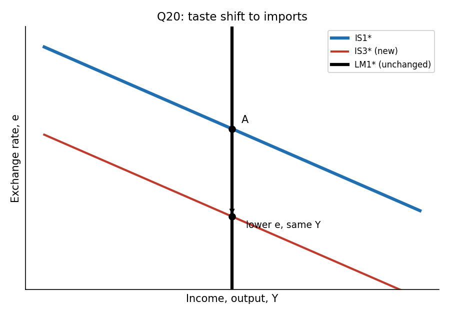
shifts down to ; with vertical , output is unchanged and falls.
- B. is a rightward shift, which would follow a fall in the taste for imports (or a tax cut).
- C and D. moves only with money supply or money demand, not with import preferences.
🗣️ In plain EnglishPeople buying more imports weakens demand for domestic goods, so the IS* curve shifts left. The currency falls to compensate, and output ends up unchanged.
Q21 — Import quota under a fixed exchange rate
Question. In a small open economy with a fixed exchange rate, if the government imposes an import quota, then net exports:
- A. increase, the money supply increases, and income increases
- B. decrease but the money supply falls and income falls
- C. are unchanged but the money supply falls and income falls
- D. are unchanged, the money supply is unchanged, and income is unchanged
AI-written answer, not official. Check before relying on it.Consistent with the tofes 0 layout (answer printed first).
Answer: A (AI-solved)
The quota raises net exports at any exchange rate, so shifts right. With the exchange rate fixed, the rightward shift creates pressure to appreciate. To defend the peg the central bank buys foreign currency and sells domestic currency, so the money supply rises and shifts right as well. In the new equilibrium income is higher and, since is unchanged, net exports end up higher than before. See Fixed Exchange Rate.
- B. Wrong sign on every item: the quota raises and pushes the money supply up.
- C. Net exports do not stay unchanged: the quota raises them. (In the floating case NX would be unchanged, because the exchange rate absorbs the shock.)
- D. That is the floating-rate result (the exchange rate absorbs the shock, and unchanged, though even there NX is unchanged only because moves). Under a fixed rate the central bank must accommodate.
🗣️ In plain EnglishUnder a fixed rate, protection works: the central bank has to print money to hold the peg, so income rises and net exports rise too. Under a floating rate the currency would absorb it all.
Q22 — Why inflation can be inertial
Question. Inflation might be inertial because
- A. people have adaptive expectations, because of which they base their future inflation expectations on the recently observed inflation
- B. people have adaptive expectations, so for example if prices have been rising quickly, people will expect them to stop rising quickly
- C. people have rational expectations, because of which they base their future inflation expectations on the recently observed inflation
- D. people have rational expectations, so for example if prices have been rising quickly, people will expect them to stop rising quickly
AI-written answer, not official. Check before relying on it.Consistent with the tofes 0 layout (answer printed first).
Answer: A (AI-solved)
Inflation Inertia comes from Adaptive Expectations: . Last period's inflation becomes this period's expectation, which feeds into wage and price setting, so inflation persists unless unemployment moves away from the natural rate.
- B. Adaptive expectations mean people expect fast inflation to continue, not stop.
- C. Mislabels: basing expectations on the recent past is adaptive, not rational. Rational Expectations use all available information.
- D. Wrong label and an example that would, if anything, remove inertia.
🗣️ In plain EnglishIf people simply expect tomorrow's inflation to look like yesterday's, inflation keeps going on its own momentum.
Q23 — Demand-pull versus cost-push
Question. The difference between demand-pull inflation and cost-push inflation is that the demand-pull inflation
- A. is due to an increase in demand which pulls output and prices up; whereas adverse shock to supply pushes up the cost of production
- B. is not expressed within the Phillips curve, whereas the cost-push inflation is expressed by the random shock, .
- C. is transitory whereas the cost-push inflation is sustainable
- D. tend to be more moderate in comparison to cost-push inflation.
AI-written answer, not official. Check before relying on it.Consistent with the tofes 0 layout (answer printed first).
Answer: A (AI-solved)
Demand-Pull Inflation starts on the demand side: AD shifts right, pulling output and prices up (it appears in the Phillips Curve as low unemployment, ). Cost-Push Inflation starts on the supply side: an adverse Supply Shock pushes up production costs ().
- B. Wrong: demand-pull is in the Phillips curve, through the term .
- C. Neither is transitory or permanent by nature. Persistence depends on expectations and the policy response.
- D. Nothing in the theory says one is milder.
🗣️ In plain EnglishDemand-pull: too much spending pulls prices up. Cost-push: higher costs push prices up.
Q24 — Phillips curve arithmetic
Question. The economy has the Phillips curve: . Unemployment has increased by 2% above its normal rate. What happened to the inflation?
- A. Inflation declined by 1%
- B. Inflation rose by 1%
- C. Inflation declined by 2%
- D. Inflation rose by 2%
AI-written answer, not official. Check before relying on it.Consistent with the tofes 0 layout (answer printed first).
Answer: A (AI-solved)
The natural rate is 5%, so "2% above its normal rate" means .
Inflation declines by 1 percentage point. The sacrifice-ratio logic is the same (Sacrifice Ratio): high unemployment brings inflation down.
- B and D. Wrong sign: high unemployment lowers inflation.
- C. Forgets the 0.5 coefficient ().
🗣️ In plain EnglishUnemployment 2 points above normal, times the slope 0.5, pulls inflation down by 1 point.
Q25 — Unexpected monetary contraction (figure)
Question. Address the following figure (price against output ; vertical LRAS at ; three SRAS and three AD curves; labelled points A (, ), B (, ), C (, ), D, E, F, G). Starting from long-run equilibrium at A with output equal to and the price level equal to , if there is an unexpected monetary contraction, then the long-run neutrality of money is represented by the movement from A to:
- A. B
- B. G
- C. C
- D. D
AI-written answer, not official. Check before relying on it.Consistent with the tofes 0 layout (answer printed first). I read the figure image: passes through G and B, through G, A and E, and through B and D.
Answer: A (AI-solved)
A monetary contraction shifts AD left (). With sticky prices (unexpected, so does not move yet) the short-run outcome is A to G: lower price, lower output. Over time prices fall further, SRAS shifts down/right (), and the economy slides along to B: output back at and the price level lower, at . That return to with only the nominal variable () changed is Money Neutrality (LR).
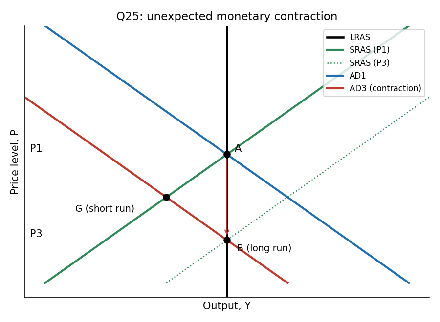
Redrawn schematic of the paper's figure: A to G in the short run, G to B in the long run.
- B (G). The short-run point, where real output still falls. Not neutrality.
- C. Above : a price rise, the long-run outcome of a monetary expansion.
- D. The intersection of and : output above at a lower price. It would follow a favourable supply shift with no demand change, not a monetary contraction.
🗣️ In plain EnglishA surprise money cut first hurts output (point G). Once prices fall enough, output returns to normal at a lower price level (point B). That is money neutrality.
Recap
| Q | Topic | Answer | Source |
|---|---|---|---|
| 1 | Solow, | A | AI-solved |
| 2 | Higher saving, short run | A | AI-solved |
| 3 | Higher raises | A | AI-solved |
| 4 | Persistent growth in steady state | A | AI-solved, flag |
| 5 | Return to capital fixed | A | AI-solved |
| 6 | Below golden rule, cut capital taxes | A | AI-solved |
| 7 | Fed vs demand shock | A | AI-solved |
| 8 | LR money neutrality | A | AI-solved |
| 9 | Okun, | A | AI-solved, flag |
| 10 | Multiplier 1 and 5 | A | AI-solved |
| 11 | Liquidity preference | A | AI-solved |
| 12 | from 6 to 4 | A | AI-solved |
| 13 | IS-LM link | A | AI-solved |
| 14 | up: up, up | A | AI-solved |
| 15 | Poole: fixed vs fixed | A | AI-solved |
| 16 | LM shift vs AD | A | AI-solved |
| 17 | Balanced budget | A | AI-solved |
| 18 | Capital inflow | A | AI-solved |
| 19 | Cut lowers | A | AI-solved |
| 20 | Import taste: IS1* to IS3* | A | AI-solved |
| 21 | Fixed-rate quota | A | AI-solved |
| 22 | Adaptive expectations | A | AI-solved |
| 23 | Demand-pull vs cost-push | A | AI-solved |
| 24 | A | AI-solved | |
| 25 | A to B | A | AI-solved |
Related notes
Macro-Economics II · PP_02-Solow, IS-LM, Mundell-Fleming & Phillips Curve (2021 Moed A) · PP_07-IS-LM, Mundell-Fleming, AS-AD & Classical Theory (2024 Moed B)