
Macro II Moed A 2023 (7 July 2023), Worked Solutions
- #macro-economics-ii
- #past-paper
- #worked-solution
- #multiple-choice
- #classical-model
- #solow
- #is-lm
- #mundell-fleming
- #as-ad
Macro II Moed A 2023: Worked Solutions
Part of: Macro-Economics II Moed A, 7 July 2023, Macroeconomics II (3058), Dr. Alon Cohen. 25 multiple-choice questions, 4% each, open notes. Builds on: Lec_03-Classical Theory & National Income, Lec_04-The Monetary System, Lec_05-Inflation, Lec_06-AS-AD Model & Economic Fluctuations, Lec_07-Aggregate Demand I & the IS-LM Model, Lec_08-Aggregate Demand II & Applying the IS-LM Model, Lec_09-The Open Economy Revisited & Mundell-Fleming Model, Lec_14-Aggregate Supply & the Phillips Curve
AI-solved questions: Q4, Q5, Q6, Q7The official answer key skips the four Solow growth questions (Q4 to Q7). Those four were solved by an AI, not taken from an official key, and each carries its own warning. The vault has no Solow lecture deck (Solow is textbook Ch 8-9), so they are grounded in the standard Solow steady-state conditions only. Check them before relying on them. Every other answer follows the official key.
What this paper tests
| Block | Questions | Core idea |
|---|---|---|
| Classical long run and money | Q1 to Q3 | Saving equals investment; the Quantity Theory of Money and the Fisher Effect |
| Growth | Q4 to Q8 | Solow steady state, golden rule, two-sector endogenous growth |
| AS-AD and the multiplier | Q9 to Q11 | Supply shocks, SR to LR price adjustment, the Keynesian Cross |
| IS-LM | Q12 to Q15 | Monetary and fiscal policy, Crowding Out, where the AD slope comes from |
| Mundell-Fleming | Q16 to Q21 | Capital mobility, floating versus fixed regimes, risk premium, large economy |
| Aggregate supply | Q22 to Q25 | Money neutrality, sticky prices, inflation inertia, long-run Phillips curve |
The one habit that wins this examAlways ask which run and which regime. Short run means prices are fixed and output moves; long run means output is back at and only prices move. In Mundell-Fleming, floating means is vertical and income is pinned by money; fixed means is horizontal and the exchange rate is pinned.
Q1 — Tax cut in the classical model
Question. Assume the classic theory, which describes a closed macroeconomy in the long run. GDP is 5,000, and . The government cuts taxes by 200 (without changing its expenditure level). What happened to the investment level?
- A. Decreased by 120
- B. Decreased by 200
- C. Increased by 120
- D. Did not change
Answer: A.
Output is fixed at (the Production Function sets it). Investment is whatever national saving leaves over, since in the Loanable Funds Market.
Before: , so .
After (): , so .
Split into parts: public saving falls by 200, private saving rises by 80 (disposable income rises by 200, of which 0.6 is spent, so only 0.4 of 200 is saved). Net: .
Why the other options are wrong
- B (down 200): counts only the fall in public saving and forgets households save 40% of the extra disposable income.
- C (up 120): right size, wrong sign. Consumption rises by 120 but that comes out of saving, it does not add to investment.
- D (no change): this is Ricardian equivalence (households save the whole tax cut). Here consumption depends on current only, so it does not hold. Lower national saving raises the real interest rate and Crowding Out reduces investment.
🗣️ In plain EnglishThe government cuts taxes but spends the same, so it borrows more. Households only save 40% of the tax cut, so total national saving falls by 120, and with less saving there is less to lend to firms, so investment drops by 120.
Q2 — Announced future money growth
Question. If the Fed announces that it will raise the money supply in the future but does not change the money supply today,
- A. both the nominal interest rate and the current price level will increase.
- B. the nominal interest rate will decrease and the current price level will increase.
- C. the nominal interest rate will increase and the current price level will decrease.
- D. both the nominal interest rate and the current price level will decrease.
Answer: A.
- Higher future money growth means higher expected inflation .
- By the Fisher Effect, , so the nominal rate rises today, even though has not moved.
- A higher is a higher cost of holding money, so Money Demand falls.
- Real balances demanded fall, but is unchanged. The market only clears if falls, so the current price level rises.
Why the other options are wrong
- B: a falling contradicts the Fisher effect; expected inflation went up, not down.
- C: rises correctly, but a falling would raise real balances and make the excess supply of money worse.
- D: wrong on both. Only a contractionary announcement would lower both.
🗣️ In plain EnglishPeople hear that more money is coming, so they expect higher inflation and lenders demand a higher nominal interest rate right away. Nobody wants to hold cash when it is about to lose value, so prices jump up today.
Q3 — Money growth and the nominal rate
Question. According to the quantity theory and the Fisher equation, if the money growth increases by 3 percent and the real interest rate equals 2 percent, then the nominal interest rate will increase:
- A. 5%
- B. 6%
- C. 3%
- D. 2%
Answer: C.
In growth rates, the Quantity Theory of Money gives . With and growth unchanged, 3 points more money growth gives 3 points more inflation, so . The real rate does not move (it is set in the loanable funds market), so
Why the other options are wrong
- A (5%): adds the 2% real rate to the change. The real rate is a level already inside , not something added to a change.
- B (6%): double counts the 3%.
- D (2%): this is just the level of the real rate, which is unaffected.
🗣️ In plain EnglishThe real rate stays at 2%, so whatever extra inflation the printing press creates passes one-for-one into the nominal rate: 3 points more inflation, 3 points more nominal rate (the Fisher effect).
Q4 — Optimal saving rate (Solow, golden rule)
Question. If an economy with no population growth or technological change has a steady-state MPK of 0.125, a depreciation rate of 0.1, and a saving rate of 0.225, then the optimal saving rate, which induces maximum consumption per worker, is
- A. higher than 0.225
- B. lower than 0.225
- C. 0.225
- D. Either higher or lower than 0.225
AI-written answer, not official. Check before relying on it.The official key skips this question. It is a Solow growth question (Ch 8-9) and there is no lecture deck for Solow in this vault, so this is solved from the standard golden-rule condition only.
Answer: A.
With , steady-state consumption per worker is . The golden rule maximises this, which requires
Here . An extra unit of capital would add 0.125 of output but only cost 0.1 of depreciation, so net consumption would rise. The economy has too little capital, so the saving rate must rise to reach the golden rule.
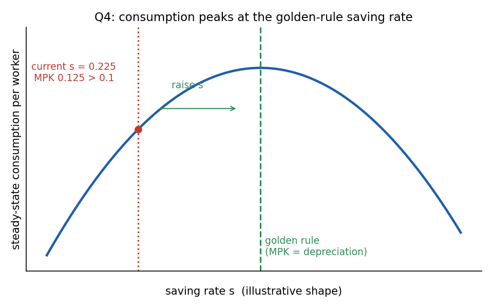
The hump is an illustrative shape. The economy sits on the rising side (MPK above depreciation), so raising raises steady-state consumption.
IntuitionSaving more costs consumption today but builds a larger capital stock. Beyond the golden rule the extra capital earns less than it wears out (MPK below depreciation), so you would be saving for nothing. Below it, as here, more saving pays.
Why the other options are wrong
- B (lower): this is the case MPK below (over-accumulation, dynamic inefficiency). The numbers are the other way round.
- C (0.225): would need MPK exactly.
- D (either): the MPK comparison pins down the direction uniquely.
🗣️ In plain EnglishCapital earns 12.5% a year but only wears out at 10%, so the economy is under-saving. To get the most consumption in the long run it should save more than 0.225.
Q5 — Growth rates of capital and the rental price (Solow)
Question. In the Solow growth model of an economy with population growth at rate , technological change at rate and capital depreciates at rate , total capital grows at rate ______ and real rental price grows at rate ______.
- A. ; 0
- B. ;
- C. ;
- D. ; 0
AI-written answer, not official. Check before relying on it.The official key skips this question (Solow, Ch 8-9, no lecture deck in the vault).
Answer: A.
In steady state, capital per effective worker is constant, so total capital grows with effective labor : .
The real rental price of capital equals the marginal product of capital, . With constant, is constant, so it grows at 0. (The real wage is the one that grows, at .)
Why the other options are wrong
- B: gets capital right but gives the rental price the growth rate of the wage. The wage grows at because and grows; the return to capital does not.
- C: depreciation is not a growth rate of the stock. It is subtracted in and cancels with gross investment, so net capital growth is still .
- D: capital does not grow at the depreciation rate.
🗣️ In plain EnglishIn the long run the capital stock grows as fast as the effective workforce (), so the return on each unit of capital stays flat (growth 0). Only wages keep growing.
Q6 — Saving rate consistent with steady-state growth (Solow)
Question. If the U.S. production function is Cobb-Douglas with capital share 0.3, total output growth is 3 percent per year, technological change rate is , population growth rate is 1%, depreciation is 4 percent per year, and the capital-output ratio is 2.5, the saving rate that is consistent with steady-state growth is:
- A. 17.5%
- B. 20%
- C. 12.5%
- D. 14%
AI-written answer, not official. Check before relying on it.The official key skips this question (Solow, Ch 8-9, no lecture deck in the vault).
Answer: A.
In steady state, total output grows at , so and .
Steady-state investment equals break-even investment: , so
Why the other options are wrong
- B, C and D (20%, 12.5%, 14%): none follows from with . Common slips are forgetting (then , which is option C) or taking from total growth without subtracting .
- The capital share 0.3 is a distractor here. It matters for and the golden rule, not for this accounting identity.
🗣️ In plain EnglishTo keep a 2.5 : 1 capital-to-output ratio while the economy grows, you need to replace what wears out (4%) and add capital for new workers and better technology (3%). That is 7% of capital per year, and 7% of is 17.5% of .
Q7 — Real wage growth (Solow)
Question. If total GDP grows 5% per year, labor force grows at 2% a year, depreciation rate is 4%, what is the real wage annual growth rate according to the Solow model?
- A. 3%
- B. 5%
- C. 6%
- D. 2%
AI-written answer, not official. Check before relying on it.The official key skips this question (Solow, Ch 8-9, no lecture deck in the vault).
Answer: A.
In steady state total output grows at , so and . The real wage grows at (output per worker grows at and the wage tracks it), so it grows at 3%.
Why the other options are wrong
- B (5%): that is total output growth, which includes labor force growth.
- C (6%): is not produced by any steady-state formula. Depreciation is a distractor and does not affect the steady-state growth rate.
- D (2%): that is the labor force growth rate, which raises total output but not output per worker.
🗣️ In plain EnglishTotal growth of 5% includes 2% from more workers. What is left, 3% a year, is better technology, and that is what raises each worker's wage.
Q8 — What makes the two-sector model endogenous
Question. Which of the following makes the two-sector model an endogenous growth theory rather than exogenous growth theory (as in Solow model)?
- A. The fraction of labor in universities,
- B. The saving rate,
- C. Both the fraction of labor in universities, , and the saving rate
- D. The labor force growth rate,
Answer: A.
In the two-sector model, knowledge (efficiency of labor) grows at , where is the share of labor working in universities. Because is a choice variable inside the model, long-run growth is determined by decisions, not by an outside constant as in Solow.
Why the other options are wrong
- B and C: the saving rate raises the level of income per worker (as in Solow) but does not change the long-run growth rate here.
- D: labor force growth is exogenous in both models.
🗣️ In plain EnglishIn Solow, technology just falls from the sky. In the two-sector model it comes from how many people we put into universities, so a society can choose its own growth rate.
Q9 — A one-year drought
Question. Assume that the economy starts at point A and there is a drought that severely reduces agricultural output in the economy for just one year. In this situation, point ______ represents the short-run equilibrium immediately following the drought and point ______ represents the eventual long-run equilibrium.
The diagram has at , a downward-sloping through A, and three horizontal lines: (top, through B and C), (through A) and (bottom, through D and E).
- A. B; A
- B. B; C
- C. E; D
- D. D; A
Answer: A.
A drought is an adverse supply shock that shifts up to . Prices are sticky, so the economy moves along to its intersection with , which is B: higher , lower (Stagflation). The shock lasts only a year, so returns to and the economy goes back to A.
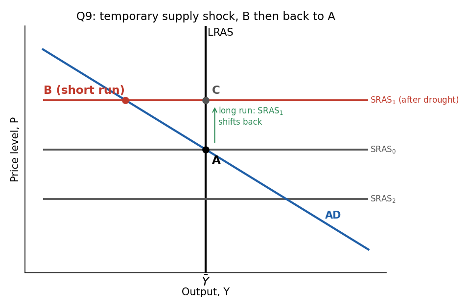
Redrawn from the exam diagram. B is on at the higher price; A is the original equilibrium.
Why the other options are wrong
- B (B; C): C is where crosses . It is not on the AD curve, so it is never an equilibrium. The shock is temporary, so there is no reason to end at a higher price level.
- C (E; D) and D (D; A): D and E sit on the lower line , which is what a favourable supply shock (a bumper harvest) would produce. A drought moves up, not down.
🗣️ In plain EnglishA drought makes goods scarcer and pricier while output falls (point B). Once the harvest returns to normal next year, everything snaps back to where it started (point A).
Q10 — Long-run adjustment of the price level
Question. Assume that the normal output level is 3,000, prices in the short run are set at , money supply is and the aggregate demand is given by . What will happen in the long run?
- A. Price level will rise by 33.33%
- B. Output increases to 4,000
- C. Money supply falls to 1,500
- D. Aggregate demand reduces to
Answer: A.
Short run (): . Output is above normal, so prices rise until returns to :
The price level rises from 1 to 4/3, an increase of 33.33%.
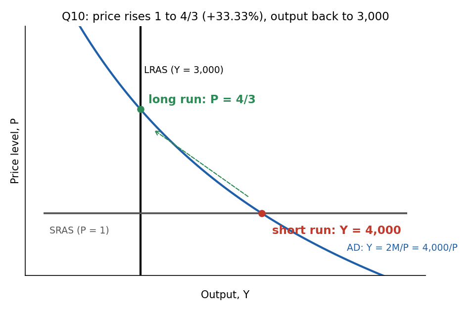
The economy starts at on the line and slides up to , where it meets .
Why the other options are wrong
- B (4,000): that is the short-run output. In the long run output is at .
- C (M falls to 1,500): is a policy variable, nothing in the model makes it fall. Note that 1,500 would give at , which is a different way to reach , but it needs the central bank to act.
- D (): the AD function is given and does not change by itself. would again give at , but only if demand fell.
🗣️ In plain EnglishDemand is too hot (4,000 versus a normal 3,000), so firms raise prices until demand cools to normal. The price needs to go from 1 to 1.33, a 33% rise, and output ends up back at 3,000.
Q11 — Why fiscal policy has a multiplier
Question. In the Keynesian-cross model, fiscal policy has a multiplied effect on income because fiscal policy:
- A. changes income, which changes consumption, which further changes income.
- B. increases the amount of money in the economy.
- C. is government spending and, therefore, more powerful than private spending.
- D. changes the interest rate.
Answer: A.
The Keynesian Cross multiplier is a feedback loop: more , and so on. Summing the geometric series gives
Why the other options are wrong
- B: the Keynesian cross has no money market. Fiscal policy does not create money.
- C: a dollar of government spending is not special. Any autonomous change in spending (for example investment) has the same multiplier.
- D: interest rates enter only when you move to IS-LM, and there they reduce the multiplier (crowding out).
🗣️ In plain EnglishThe government spends a dollar, someone earns it, spends most of it, and the next person earns that. The income keeps getting passed on, so the total effect is bigger than the original dollar.
Q12 — Monetary expansion and the nominal rate
Question. In the money market, monetary expansion leads to ______ nominal interest rate in the short run (when is fixed), and to ______ nominal interest rate in the long run.
- A. Lower, higher
- B. Lower, lower
- C. Higher, lower
- D. Higher, higher
Answer: A.
Short run ( fixed): means . There is an excess supply of real balances, people buy bonds, bond prices rise and falls (the liquidity effect).
Long run: money is neutral, so rises in proportion to and returns to its original level. The real rate is unchanged, but a sustained higher money growth rate means higher inflation, so by the Fisher Effect the nominal rate is higher.
Why the other options are wrong
- B: gets the SR right but forgets the Fisher effect in the LR.
- C and D: a higher short-run rate would need money demand to rise or money supply to fall, which is the opposite of an expansion.
🗣️ In plain EnglishAt first more money means more cash chasing bonds, so rates fall. Over time prices catch up and inflation expectations rise, which pushes nominal rates above where they started.
Q13 — Full multiplier in IS-LM
Question. In the IS-LM model, following an increase of government expenditure by , output level has risen by . What happened to the level of investment in this transition?
- A. Investment has not changed
- B. Investment has increased
- C. Investment has decreased
- D. Investment could have either increased or decreased
Answer: A.
In general, , where is the change in investment caused by the interest-rate response. If rose by exactly , then , so the interest rate did not move (for example the central bank accommodates, or is flat).
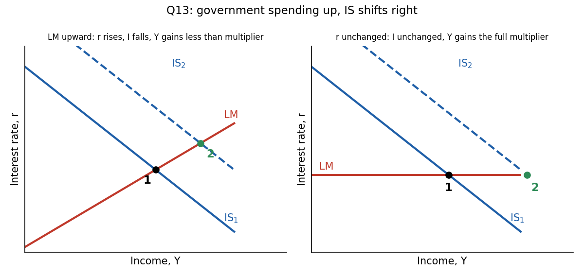
Left: an upward means rises, Crowding Out cuts , and rises by less than the multiplier. Right: with unchanged the full Keynesian-cross multiplier is realised.
Why the other options are wrong
- B (increased): a rise in would push above . A fiscal expansion cannot lower on its own.
- C (decreased): the usual case, but then would rise by less than the multiplier.
- D (either): the exact value pins down .
🗣️ In plain EnglishNormally the government soaks up savings and pushes interest rates up, which squeezes out private investment and the boost is smaller. If income rose by the full textbook multiplier, nothing can have been squeezed out, so investment did not change.
Q14 — Bond sell-off
Question. When traders massively sell bonds, the interest rate ______, which shifts the ______ curve to the left.
- A. rises, LM
- B. falls, LM
- C. rises, IS
- D. falls, IS
Answer: A.
Heavy bond selling pushes bond prices down, so yields (the interest rate) rise. Traders are swapping bonds for cash, so money demand rises. At each income level a higher is needed to keep the money market in equilibrium, so the LM Curve shifts left.
Why the other options are wrong
- B and D: falling prices of bonds mean rising, not falling, yields.
- C and D (IS): the IS curve describes goods-market equilibrium, which is not what a portfolio shift between bonds and cash changes. Also, an IS shift to the left would lower .
🗣️ In plain EnglishEveryone dumping bonds for cash makes bonds cheaper, so their yield (the interest rate) goes up. People wanting more cash is a money-market story, so the LM curve moves, not IS.
Q15 — Why the AD curve slopes down (IS-LM)
Question. Based on the IS-LM model, what is the explanation for the downward slope of the AD curve?
- A. The interest rate effect
- B. The exchange rate effect
- C. The price effect
- D. All answers are correct
Answer: A.
In IS-LM: shifts left . This is the interest-rate effect, and it is what gives the Aggregate Demand Curve its negative slope.
Why the other options are wrong
- B: the exchange-rate effect (higher appreciates the currency and lowers net exports) appears in the open-economy derivation of AD, not in closed-economy IS-LM.
- C: "the price effect" is not a mechanism in this course.
- D: so not all are correct.
🗣️ In plain EnglishA higher price level shrinks the real value of the money supply, which pushes interest rates up, which discourages investment and lowers output. That is why demand falls as prices rise.
Q16 — Free capital mobility
Question. When residents of a small economy can freely save their funds abroad or borrow funds from abroad then
- A. When domestic interest rate is lower than the world interest rate, net capital outflow increases
- B. When domestic interest rate is higher than the world interest rate, net capital outflow increases
- C. Real exchange rate is 1 in the short run.
- D. Domestic price level equals the world price level
Answer: A.
With perfect Capital Mobility, if residents earn more by lending abroad, so net capital outflow rises, driving back up to .
Why the other options are wrong
- B: reversed. If foreign funds flow in, outflow falls.
- C and D: capital mobility concerns financial assets, not goods. It does not force purchasing-power parity, so the real exchange rate need not equal 1 and price levels may differ.
🗣️ In plain EnglishIf you can earn more abroad than at home, you send your savings abroad. That outflow continues until the home rate is pushed back to the world rate.
Q17 — What depreciates the currency (floating)
Question. In a small open economy with a floating exchange rate, the exchange rate will depreciate if:
- A. Taxes are raised
- B. government spending is increased
- C. Taxes are cut
- D. the money supply is decreased
Answer: A.
Under floating rates (Mundell-Fleming Model), higher taxes reduce consumption and shift left. is vertical, so is unchanged and the exchange rate falls (depreciates).
Why the other options are wrong
- B and C: both shift right, so the currency appreciates.
- D: a lower money supply shifts left, raising (appreciation) and lowering .
🗣️ In plain EnglishHigher taxes mean less spending at home, so less demand for the currency to buy things with, and the currency falls. Output stays put because the money supply is what fixes it.
Q18 — Horizontal and import restrictions
Question. In the Mundell-Fleming model, suppose that the is perfectly horizontal. This is consistent with a ______ exchange rate regime, which makes restrictions on import ______ policy in attempt to boost economic activity.
- A. Fixed, effective
- B. Fixed, ineffective
- C. Floating, effective
- D. Floating, ineffective
Answer: A.
A horizontal LM* Curve means the central bank adjusts to hold constant, which is a Fixed Exchange Rate. Import restrictions shift right. Pressure to appreciate forces the central bank to expand to defend the peg, so shifts right too, and rises. Trade policy is effective under fixed rates.
Why the other options are wrong
- B: fixed is right but fiscal and trade policy are effective under fixed rates (monetary policy is the one that is not).
- C and D: a floating regime has a vertical . There, import restrictions shift right but simply appreciates and is unchanged, so floating makes them ineffective (D would be half right, but it contradicts the regime named by the horizontal ).
🗣️ In plain EnglishA flat means the central bank is defending a fixed exchange rate. When it has to print money to hold the peg, the trade restriction's boost to demand is not cancelled out, so it works.
Q19 — Risk premium and income
Question. An increase in income generated by an increase in the country risk premium will not occur if there is a(n) ______ sufficient to offset the decline in the demand for money caused by the higher risk premium.
- A. increase in the price level caused by more expensive imports
- B. fall in the price level caused by less expensive imports
- C. decrease in government spending
- D. increase in the money supply
Answer: A.
A higher Country Risk Premium raises the domestic rate () and depreciates the currency. The higher lowers money demand, shifting right and raising . But a depreciation makes imports dearer, so the domestic price level rises, falls and shifts back left, offsetting the income gain.
Why the other options are wrong
- B: depreciation makes imports more expensive, not cheaper. Also a fall in would raise and add to the expansion.
- C: under floating rates is set by . A cut in moves only (and ), so it cannot cancel an -driven rise in .
- D: more money shifts further right, increasing even more.
🗣️ In plain EnglishA scarier country means higher interest rates and a weaker currency, which would normally lift income. But a weak currency makes imports costlier, so prices rise, which eats into the money supply in real terms and cancels the boost.
Q20 — Monetary expansion in a large open economy
Question. In a large open economy, monetary expansion increases output level in the short run due to
- A. Both the interest rate effect and the exchange rate effect
- B. Only the interest rate effect
- C. Only the exchange rate effect
- D. Neither the exchange rate effect nor the interest rate effect
Answer: A.
A Large Open Economy is a hybrid of the closed and small-open cases. Expansion lowers , which raises (interest-rate channel). Lower relative to the world also causes capital outflow and a depreciation, which raises net exports (exchange-rate channel). Both boost .
Why the other options are wrong
- B: is the closed-economy story. It ignores the exchange-rate channel.
- C: is the small-open-economy story. Here the interest rate falls too, because the economy is large enough to move .
- D: contradicts the fact that output rises.
🗣️ In plain EnglishMore money lowers interest rates, so firms invest more, and the cheaper currency makes our goods more competitive abroad. A large economy gets both boosts.
Q21 — Preference shift towards foreign cars
Question. The introduction of a stylish new line of Toyotas, which makes some consumers prefer foreign cars over domestic cars, will, according to the Mundell-Fleming model with floating exchange rates, lead to:
- A. no change in income or net exports.
- B. a fall in income and net exports.
- C. a fall in income but no change in net exports.
- D. no change in income but a fall in net exports.
Answer: A.
Net exports fall at every exchange rate, so shifts left. With floating rates and a vertical , is unchanged and depreciates. The depreciation makes domestic goods cheaper and restores the original level of . Since , , and are all unchanged, the national income identity forces to be unchanged too.
Why the other options are wrong
- B and C: a fall in needs a shift in , and here it did not move.
- D: (equivalently ). With nothing else changing, cannot change.
🗣️ In plain EnglishPeople want foreign cars, so the currency weakens. A weaker currency makes our products attractive again, and in the end income and trade balance are exactly where they started. The only thing that moved is the exchange rate.
Q22 — Unexpected monetary expansion
Question. Starting from long-run equilibrium at A with output equal to and the price level equal to , if there is an unexpected monetary expansion that shifts aggregate demand from to , then the equilibrium
- A. will change to E in the short run, reflecting money non-neutrality, and C in the long run, reflecting money neutrality
- B. will change to E in the short run, reflecting money neutrality, and C in the long run, reflecting money non-neutrality
- C. will change to C in the short run, reflecting money non-neutrality, and E in the long run, reflecting money neutrality
- D. will change to C in the short run, reflecting money neutrality, and E in the long run, reflecting money non-neutrality
Answer: A.
The expansion is unexpected, so and the curve () does not move at first. meets at E, where and is higher. Output moves in response to a nominal change, so money is non-neutral in the short run.
Later, expectations catch up, rises and shifts up. The economy settles where meets at C: , only is permanently higher (Money Neutrality (LR)).
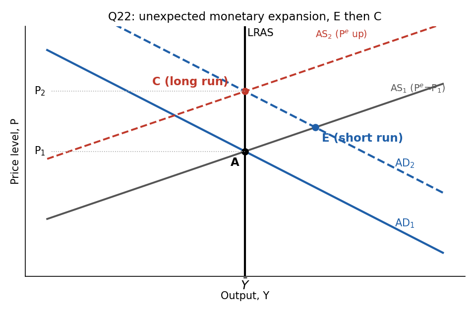
Simplified redrawing of the exam diagram (the original also shows , and points B, D, F, G, which are not needed). E is on and ; C is on and .
Why the other options are wrong
- B: has the neutrality labels the wrong way round. Moving in the SR is non-neutrality.
- C and D: C is on , so it can only be the long-run point, never the short-run one.
🗣️ In plain EnglishSurprise money creation boosts output for a while because prices and expectations are slow to adjust (point E). Once everyone catches on, only prices end up higher and output goes back to normal (point C).
Q23 — Why SRAS slopes upward
Question. A possible reason that the AS slopes upward in the short run, and is not perfectly horizontal, is that
- A. Some of the firms' prices are flexible
- B. Price expectations could differ from actual prices in the short run
- C. Price expectations could differ from actual prices in the long run
- D. When output exceeds its normal rate some of the firms cannot respond by raising their prices as they would like to
Answer: A.
In the Sticky-Price Model, a fraction of firms have flexible prices and adjust right away, and the rest are sticky. If all prices were sticky, would be horizontal. The flexible-price firms raise prices when demand rises, so the average price level rises a little and the curve slopes up. More flexible firms mean a steeper SRAS Curve.
Why the other options are wrong
- B: this is a real driver of the SRAS equation and is the closest competitor to A. But the question contrasts "upward-sloping" with "perfectly horizontal", which is the sticky-versus-flexible distinction, and the key chooses A. If your lecturer's notes frame B as correct, note the ambiguity.
- C: in the long run expectations adjust and is vertical, so this does not explain a short-run slope.
- D: firms that cannot raise prices make the curve flatter, not steeper. It is the opposite of what the question needs.
🗣️ In plain EnglishIf no one could change prices, the curve would be flat. But some firms do raise prices quickly when demand picks up, so the price level creeps up and the curve tilts.
Q24 — Inflation inertia in AS-AD
Question. To illustrate inflation inertia in an aggregate demand-aggregate supply model, the short-run aggregate supply curve shifts upward because of increases in ______, and the aggregate demand curve shifts upward because of increases in ______.
- A. the expected price level; the money supply
- B. the money supply; the expected price level
- C. output; the price level
- D. the price level; output
Answer: A.
With Inflation Inertia, past inflation feeds expectations. Higher expected prices shift up. To keep output from falling, the central bank expands the money supply, and since depends on , higher shifts up. The two shifts keep prices rising period after period.
Why the other options are wrong
- B: swaps the two. is a demand-side policy variable, not a shifter of .
- C and D: changes in or are movements along the curves, not shifts. and are endogenous results, not shifters.
🗣️ In plain EnglishWorkers expect more inflation, so they push prices up (supply shifts up). The central bank keeps printing money to stop output falling (demand shifts up), and inflation keeps rolling.
Q25 — No long-run inflation-unemployment tradeoff
Question. The tradeoff between inflation and unemployment does not exist in the long run. It is implied by:
- A. the classical dichotomy.
- B. Okun's law.
- C. Phillips curve.
- D. the Fisher effect.
Answer: A.
The Classical Dichotomy says real variables such as unemployment are determined independently of nominal variables such as inflation in the long run. This implies a vertical long-run Phillips curve at the Natural Rate of Unemployment: higher inflation does not buy lower unemployment.
Why the other options are wrong
- B (Okun's Law): links output gaps to unemployment, not to inflation.
- C (Phillips Curve): is the tradeoff itself (short run), not the reason it disappears. The long-run version is the one that implies no tradeoff.
- D (Fisher effect): links inflation to the nominal interest rate.
🗣️ In plain EnglishIn the long run, money and prices cannot change real things like how many people have jobs. So pushing inflation up does not permanently lower unemployment.
Recap table
| Q | Topic | Answer | One-line reason |
|---|---|---|---|
| 1 | Tax cut, classical | A | National saving falls by 120, so investment falls by 120 |
| 2 | Announced money growth | A | Expected inflation raises now, so money demand falls and jumps |
| 3 | Fisher | C | , the real rate does not move |
| 4 | Golden rule (AI-solved) | A | MPK above depreciation, so under-saving, raise |
| 5 | Solow growth rates (AI-solved) | A | grows at , the rental price (MPK) is flat |
| 6 | Steady-state saving (AI-solved) | A | |
| 7 | Real wage growth (AI-solved) | A | |
| 8 | Endogenous growth | A | Share of labor in universities |
| 9 | Drought | A | SR at B on , back to A |
| 10 | LR price level | A | , up 33.33% |
| 11 | Keynesian multiplier | A | Income to consumption to income feedback |
| 12 | Money and | A | Lower in SR (liquidity), higher in LR (Fisher) |
| 13 | Full multiplier in IS-LM | A | , no crowding out |
| 14 | Bond sell-off | A | Yield up, LM left |
| 15 | AD slope in IS-LM | A | Interest rate effect |
| 16 | Capital mobility | A | raises net capital outflow |
| 17 | Floating depreciation | A | Tax rise shifts left |
| 18 | Horizontal | A | Fixed regime, trade policy effective |
| 19 | Risk premium | A | Dearer imports raise , cutting |
| 20 | Large open economy | A | Both interest-rate and exchange-rate channels |
| 21 | Foreign-car preference | A | and both unchanged |
| 22 | Unexpected money | A | E in SR, C in LR |
| 23 | Upward SRAS | A | Some flexible-price firms |
| 24 | Inflation inertia | A | shifts SRAS, shifts AD |
| 25 | No LR tradeoff | A | Classical dichotomy |
Related notes
- Macro-Economics II (hub)
- Lec_03-Classical Theory & National Income · Lec_04-The Monetary System · Lec_05-Inflation · Lec_06-AS-AD Model & Economic Fluctuations
- Lec_07-Aggregate Demand I & the IS-LM Model · Lec_08-Aggregate Demand II & Applying the IS-LM Model · Lec_09-The Open Economy Revisited & Mundell-Fleming Model · Lec_14-Aggregate Supply & the Phillips Curve