
Macro II Moed B 2024 — Worked Solutions
- #macro-economics-ii
- #past-paper
- #worked-solution
- #multiple-choice
- #is-lm
- #mundell-fleming
- #as-ad
- #phillips-curve
- #classical-theory
- #solow
Macro II Moed B 2024 — Worked Solutions
Part of: Macro-Economics II Moed B, 30 July 2024 — Macroeconomics II (3058), Dr. Alon Cohen. 25 multiple-choice questions, 4% each, open notes. Builds on: Lec_03-Classical Theory & National Income · Lec_04-The Monetary System · Lec_05-Inflation · Lec_06-AS-AD Model & Economic Fluctuations · Lec_07-Aggregate Demand I & the IS-LM Model · Lec_08-Aggregate Demand II & Applying the IS-LM Model · Lec_09-The Open Economy Revisited & Mundell-Fleming Model · Lec_14-Aggregate Supply & the Phillips Curve
AI-solved questions: Q1, Q8, Q14, Q15The official key skips these four (all Solow growth, Ch 8-9, which has no lecture deck in this course). They are solved by me from the standard Solow model and the cheat sheet. Not official. Check before relying on them. Each is flagged again at its own question. The other 21 answers follow the official key.
What this paper tests
The paper in one paragraphAbout half the paper is short-run policy analysis, and the rest is the classical long run plus a handful of Solow questions.
- IS-LM and Keynesian cross (Q2, Q3, Q9, Q20, Q24): solve IS and LM, trace the price adjustment back to , balanced-budget multiplier, bond-buying logic of liquidity preference.
- Mundell-Fleming (Q4, Q5, Q10, Q21, Q25): floating rates (the exchange rate absorbs the shock, is fixed by LM*), fixed rates (the central bank defends the peg), large open economy.
- AS-AD and Phillips curve (Q6, Q7, Q16, Q22, Q23): shocks, short-run vs long-run adjustment, sacrifice ratio, bow-shaped SRAS.
- Classical theory and money (Q11, Q12, Q13, Q18, Q19): loanable funds, quantity theory, neutrality.
- Growth (Q1, Q8, Q14, Q15, Q17): Solow and the AK model. Q17 is the only one with an official answer.
The recurring trick: in floating-rate M-F the LM* curve is vertical, so output only moves when money or money demand moves. Fiscal and trade shocks go entirely into the exchange rate.
Q1 — Taxing savings to reach the golden rule
AI-written answer, not official. Check before relying on it.Outside the lecture notes (Solow, Ch 8-9 has no deck). Solved from the standard Solow model.
Question. In an attempt to reach the golden-rule capital level, the government has decided to impose taxes on savings. As a result,
- A. Income per person would fall
- B. Consumption will continuously increase until it reaches the new steady state level
- C. Household will increase their savings
- D. Capital per-worker will fall, and then rise above its original level
Answer: A (AI-solved)
A tax on saving lowers the saving rate . In the Solow model the steady state solves , so a lower shifts the investment curve down and steady-state falls, and with it .
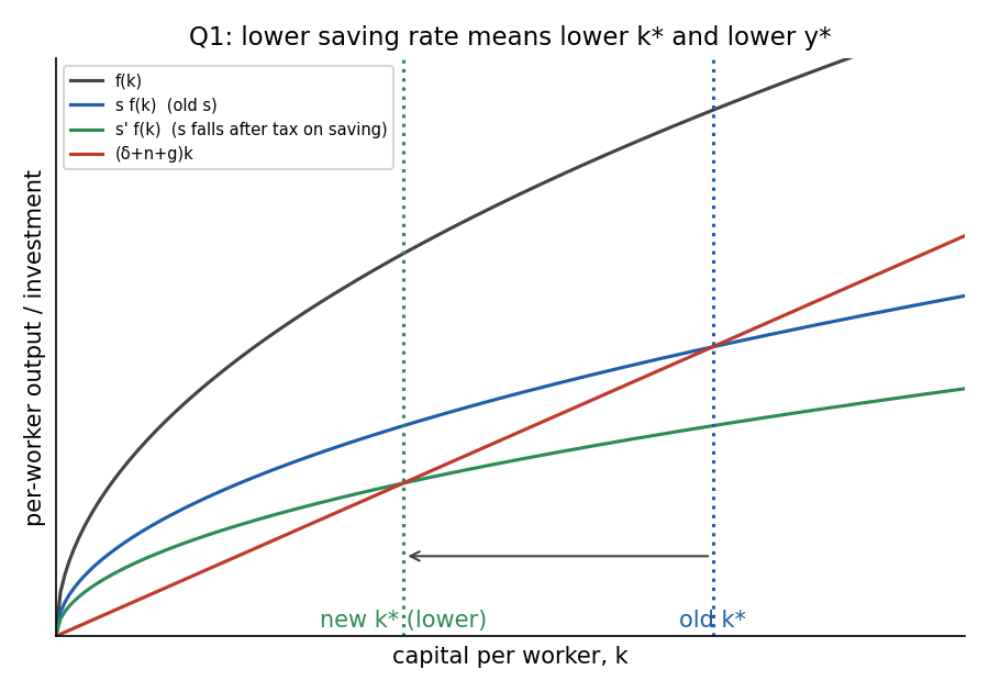
Lower moves the steady state left: less capital per worker, less income per worker.
- A. True. falls, so income per person falls (the economy was above the golden rule, so this is the price of lowering ).
- B. False. Consumption is . When falls, jumps up at once, then drifts down as and shrink toward the new steady state. It never rises continuously.
- C. False. The tax discourages saving, so households save less, not more.
- D. False. falls monotonically to a lower steady state. It never overshoots back above the old level.
IntuitionThe government's goal (golden rule) means the economy has too much capital. Cutting saving is the right direction, but it still lowers income per worker. What improves is steady-state consumption, not income.
🗣️ In plain EnglishTaxing savings makes people save less, so the economy builds up less capital and ends up with lower income per person. Consumption gets a quick boost first, then fades back.
Q2 — IS-LM with a deficit of 100
Question. Closed economy in the short run: , , , , . The government has a deficit of 100. In equilibrium
- A. ,
- B. ,
- C. ,
- D. ,
Answer: A
Step 1, taxes. Deficit , so .
Step 2, IS curve.
Step 3, LM curve. Money market clears when :
Step 4, solve. , then .
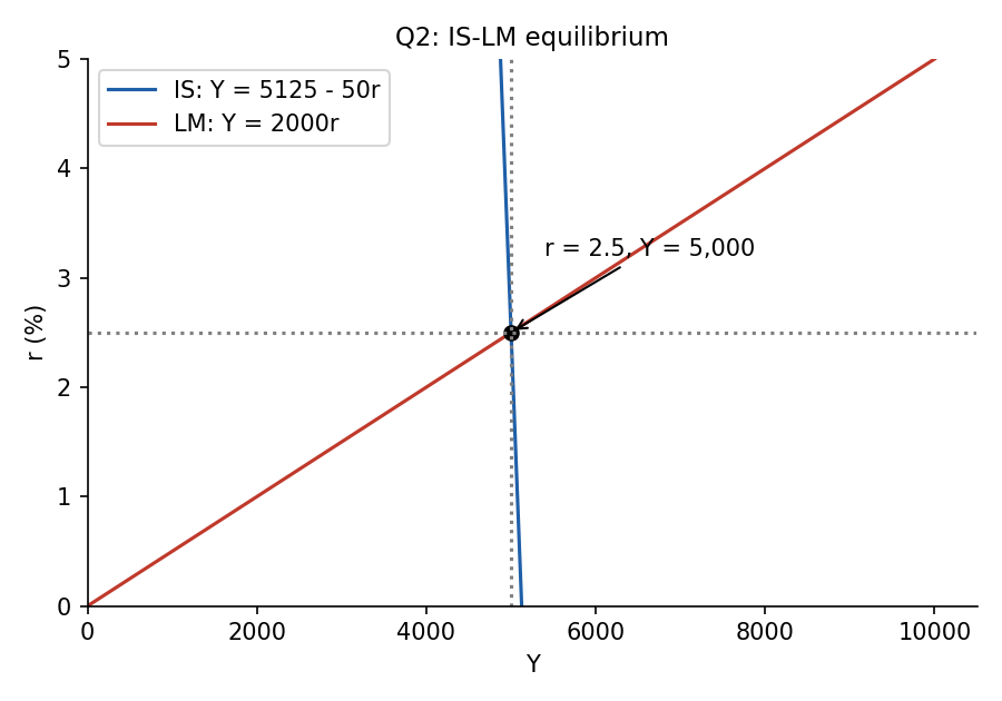
The IS curve is almost vertical because investment is only mildly sensitive to ().
Why the others fail:
- B (, ): satisfies LM () but IS gives . Not on both curves.
- C (, ): satisfies LM but IS gives .
- D (, ): LM gives and IS gives . Fits neither.
Check shortcutTest each option in both equations. Only A passes both.
🗣️ In plain EnglishFind the tax from the deficit first, then write the IS and LM lines and see where they cross. They meet at an interest rate of 2.5% and income of 5,000.
Q3 — Output above normal: the path back to the long run
Question. In the IS-LM model, output exceeds its normal level. Subsequently, in the transition towards the long run
- A. People will liquidate their bonds, thus increasing the interest rate
- B. People will liquidate their bonds, thus decreasing the interest rate
- C. Price level rises, and interest rate falls
- D. Price level falls and interest rate rises
Answer: A
means excess demand, so prices rise. A higher lowers real balances . People now hold less real money than they want, so they sell bonds to get cash. Selling bonds pushes bond prices down and the interest rate up. That is the LM curve shifting left until falls back to . See Liquidity Preference and IS-LM Equilibrium.
- B. Right mechanism (selling bonds) but wrong direction: selling bonds raises .
- C. Prices do rise, but rises too, since LM shifts left.
- D. Prices rise when , not fall.
🗣️ In plain EnglishWhen the economy is running hot, prices rise and people's cash buys less, so they sell bonds for cash. That pushes interest rates up and cools things down.
Q4 — Tax cut under floating rates (Mundell-Fleming)
Question. Mundell-Fleming, floating rate. The benchmark equilibrium is point A. The government cuts taxes. Which is the new equilibrium?
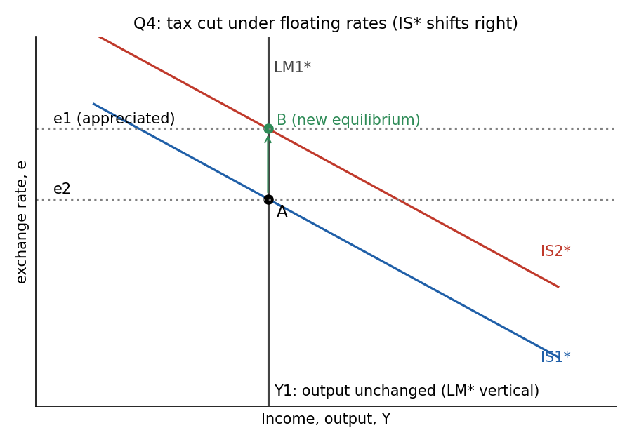
(Figure in the paper: exchange rate on the vertical axis, income on the horizontal. passes through A and D, passes through B and C. is vertical at through A and B, is vertical at through C and D. .)
- A. B, since capital inflow appreciates the exchange rate
- B. C, since capital outflow depreciates the exchange rate
- C. B, since capital inflow depreciates the exchange rate
- D. C, since capital outflow appreciates the exchange rate
Answer: A
A tax cut raises disposable income and consumption, so IS* shifts right (). Money is unchanged, so LM* stays at , vertical at . The new intersection is B: same , higher .
The mechanism: the IS shift would push the domestic rate above , which draws capital inflow, raising demand for the domestic currency, so the currency appreciates (higher ). The appreciation crowds out net exports exactly enough to leave unchanged.
- B and D (point C): C lies on , which would need a money-supply increase. A tax cut does not move LM*. Also "capital outflow" has the wrong sign.
- C (B but "inflow depreciates"): right point, wrong reasoning. Inflow raises demand for domestic currency, so it appreciates it.
See Floating Exchange Rate, IS* Curve, LM* Curve.
🗣️ In plain EnglishA tax cut under floating rates doesn't change output. It just makes the currency stronger, which hurts exports and cancels the boost.
Q5 — Fiscal expansion in a large open economy
Question. Large open economy, floating rate. The government raises spending without raising taxes. What happens to investment and net exports?
- A. Investments fall, net export falls
- B. Investments are unchanged, net export falls
- C. Investments are unchanged, net export is unchanged
- D. Investments fall, net export is unchanged
Answer: A
A Large Open Economy is an average of a closed and a small open economy. The interest rate is not pinned to .
- shifts IS right, so rises somewhat (closed-economy direction).
- Higher means falls.
- Higher also reduces capital outflow , and since , falls. The exchange rate appreciates (small-open direction).
Why the others fail:
- B and C (investment unchanged): that is the small open economy result, where is pinned. Here moves.
- C and D (NX unchanged): NX is unchanged in a small open economy under floating rates. Here and rose, so NX falls.
🗣️ In plain EnglishA big economy borrowing more pushes up its own interest rate a bit. That crowds out investment and also strengthens the currency, hurting net exports. It's a mix of the closed and small-open stories.
Q6 — Sacrifice ratio with Okun's law
Question. Short-run Phillips curve . Okun's law: 1 pp of unemployment equals 2 pp of GDP. To lower inflation by 2 pp, the central bank needs additional ____ pp of cyclical unemployment and a loss of ____ pp of GDP.
- A. 4; 8
- B. 2; 4
- C. 8; 4
- D. 4; 2
Answer: A
Cyclical unemployment. We need :
So cyclical unemployment () is 4 pp.
GDP loss. Okun: pp.
Why the others fail:
- B (2; 4): forgets the 0.5 coefficient (uses ).
- C (8; 4): halves instead of doubling in the Okun step.
- D (4; 2): right first number, but divides by 2 instead of multiplying.
See Phillips Curve, Sacrifice Ratio, Okun's Law, Cyclical Unemployment.
🗣️ In plain EnglishEach point of extra unemployment shaves half a point off inflation, so to cut inflation by 2 points you need 4 points of unemployment. Okun's law doubles that into an 8% GDP loss.
Q7 — Cost-push inflation, long-run outcome
Question. Starting from long-run equilibrium at A, a cost-push inflation would lead to long-run equilibrium in
(Figure: AS-AD diagram with vertical LRAS at . Points A, B, C lie on the LRAS at price levels , , respectively, with . Points D, E, F, G are off the LRAS. Curves AS, AS, AS and AD, AD, AD.)
- A. A
- B. B
- C. C
- D. F
Answer: A
Cost-Push Inflation is a temporary adverse supply shock: SRAS shifts up (to AS). In the short run falls and rises (Stagflation). With , wages and costs eventually fall, so SRAS drifts back down to AS. With no policy response, the economy returns to A.
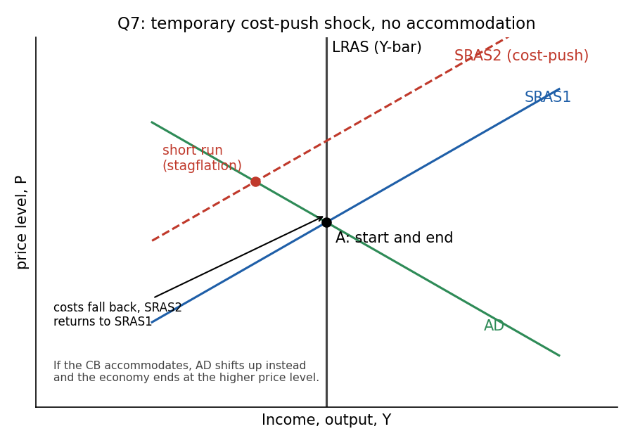
Schematic of the cost-push case, drawn from the logic of the question (not the exam's exact figure).
- B sits at a lower price level : it is the long run after a negative demand shock, not a supply shock.
- C sits at the higher price level : it is where you end if the central bank accommodates (AD shifts up to validate the price rise). The question says nothing about accommodation.
- F is off the LRAS (), so it cannot be a long-run equilibrium.
IntuitionWhether a supply shock is "temporary" depends on policy. Accommodation turns the cost shock into permanently higher prices (the 1970s lesson in the lecture).
🗣️ In plain EnglishA one-off cost shock hurts output and raises prices for a while. If the central bank just waits, costs ease and the economy drifts back to where it started.
Q8 — Returns to capital in the Solow model
AI-written answer, not official. Check before relying on it.Outside the lecture notes (Solow, Ch 8-9, no deck). Lower confidence than the other AI answers: the wording is ambiguous, see the note at the end.
Question. In the Solow model we assume a production function with ______ returns to capital, which in the steady state leads to ______ returns to capital.
- A. decreasing, fixed
- B. fixed, fixed
- C. decreasing, decreasing
- D. fixed, decreasing
Answer: A (AI-solved)
Solow assumes diminishing returns to capital (, e.g. with ). Those diminishing returns are what make growth in capital per worker die out: investment eventually equals break-even investment and stops growing. At that steady state the return to capital (MPK) is constant, so growth in is zero rather than perpetual.
- B and D assume constant returns in the production function. That is the AK model (see Q17), which has no steady state and gives permanent growth.
- C: diminishing returns remain true everywhere along the curve, so this reading is defensible, but "leads to" suggests a consequence, and the consequence of diminishing returns is a stable steady state with a fixed return.
AmbiguityIf the lecturer meant "diminishing returns are still present at the steady state", the answer would be C. I chose A because the stem frames the steady state as something diminishing returns lead to. Worth checking against the Solow slides.
🗣️ In plain EnglishSolow says each extra bit of capital adds less than the last one. That's why the economy settles down at a steady state instead of growing forever from saving alone.
Q9 — Balanced-budget multiplier
Question. Keynesian cross, fixed interest rate, MPC = 0.8. Government raises spending by $1 billion, financed by additional taxes. Planned expenditure rises by ____ and equilibrium income by ____.
- A. $0.2 billion; $1 billion
- B. $1 billion; $5 billion
- C. $0.8 billion; $1 billion
- D. $0.2 billion; $5 billion
Answer: A
Planned expenditure. . Spending rises $1B, but the tax cuts consumption by $0.8B.
Equilibrium income. Government-purchase multiplier ; tax multiplier . Sum:
The balanced-budget multiplier is exactly 1, whatever the MPC. Alternatively, .
- B (1; 5): ignores the tax entirely (treats it as a pure increase).
- C (0.8; 1): 0.8 is the consumption loss, not the net change in expenditure.
- D (0.2; 5): right first number, but then applies the pure- multiplier of 5 to the whole $1B and forgets the tax multiplier of . The correct step is .
See Keynesian Cross, Fiscal Multiplier, Marginal Propensity to Consume.
🗣️ In plain EnglishThe government spends $1B but taxes $1B, so people cut spending by 80 cents of it. Net boost to demand is 20 cents, and after the multiplier, income rises by exactly $1B.
Q10 — Import quota under floating rates
Lettering typo in the paperThe four options are lettered E, F, G, H in the exam. The official key calls the first one E. Read them as A to D.
Question. Small open economy, floating rate. The government imposes a restrictive quota on imports. As a result,
- E (first). domestic industries which sell substitutes to imported goods will benefit; but these benefits will be offset by the reduction in exports
- F (second). ... benefit; but these benefits will be offset by the increase in exports
- G (third). volume of international trade (exports plus imports) will fall, exchange rate will not change
- H (fourth). volume of international trade will not change, exchange rate will appreciate
Answer: E (the first option)
A quota raises at each , so IS* shifts right. With LM* vertical, is unchanged and appreciates. The appreciation makes exports dearer abroad, so exports fall. Imports fall directly (the quota). Net exports are unchanged (they equal , all fixed). Import-competing industries gain, but the gain is offset by lost exports.
- F: exports fall, they do not rise.
- G: trade volume does fall (both imports and exports drop), but the exchange rate does change: it appreciates.
- H: the exchange rate does appreciate, but trade volume falls, it does not stay the same.
See Floating Exchange Rate, Net Exports, Beggar-Thy-Neighbour Policy.
🗣️ In plain EnglishA quota makes the currency stronger, which hurts exporters by as much as local producers gain. Total trade shrinks and the trade balance doesn't improve.
Q11 — Households consume a larger share of income
Question. Classical theory, long-run equilibrium. Households' preferences change so they consume a larger portion of income. The interest rate
- A. rises
- B. falls
- C. is unchanged
- D. could either fall, rise or stay the same
Answer: A
Output is fixed by supply and is unchanged. National saving falls, so the supply of loanable funds shifts left. Investment demand is unchanged, so the equilibrium rises (and falls). See Loanable Funds Market, National Saving.
- B: opposite direction. Lower saving cannot lower .
- C: would need saving to be unchanged.
- D: the direction is unambiguous, because only the supply side moves and demand is downward-sloping.
🗣️ In plain EnglishIf people spend more and save less, there's less money to lend, so borrowing gets more expensive and interest rates go up.
Q12 — Bond-financed government spending and the price level
Question. Classical theory, long-run equilibrium. The government increases spending and finances it by issuing bonds. The price level
- A. rises
- B. falls
- C. is unchanged
- D. could either fall, rise or stay the same
Answer: C
Quantity theory: . Bond financing leaves unchanged, is constant and is fixed by supply, so is unchanged. The deficit only affects the real side: it lowers saving, raises and crowds out investment. See Quantity Theory of Money, Crowding Out.
- A and B: moves only if , or move. None does.
- D: tempting because crowding out is a real effect with an ambiguous-feeling story, but nothing in changes.
🗣️ In plain EnglishBorrowing by selling bonds doesn't print money, so prices stay put. It just pushes interest rates up and squeezes out private investment.
Q13 — Money now vs an announced future increase
Question. Under classical theory, if the Fed increases now, or alternatively declares it will increase next year, then
- A. money is neutral in both options
- B. neutral under the first option, but not neutral under the second
- C. not neutral under the first option, but neutral under the second
- D. not neutral in both options
Answer: A
Under the Classical Dichotomy, real variables are determined by supply-side factors, and money only moves nominal variables. Increasing now raises proportionally, real variables unchanged. Announcing a future increase raises expected inflation, which by the Fisher Effect raises the nominal interest rate () but leaves the real rate and output alone. See Money Neutrality.
- B: expectations change nominal , not real variables, so the announcement is still neutral.
- C and D: an actual money increase is the textbook neutral case.
🗣️ In plain EnglishIn the classical world money is a veil. Printing more now, or promising to print later, only changes prices and nominal rates, never real output.
Q14 — MPK/APK equals the saving rate
AI-written answer, not official. Check before relying on it.Outside the lecture notes (Solow, Ch 8-9, no deck). Solved from the standard Solow golden-rule condition. Wording is loose, see the caveat.
Question. Solow model where the ratio of the marginal product of capital to the average product of capital equals the saving rate. We can conclude that
- A. consumption is maximized
- B. consumption is not maximized
- C. consumption could be either maximized or not maximized
- D. saving rate is minimized
Answer: A (AI-solved)
At a steady state, , so , where . The golden-rule condition is . Dividing both sides by :
So is exactly the golden-rule condition, which maximizes steady-state consumption. For Cobb-Douglas, , so this is the familiar .
- B: contradicts the golden-rule condition.
- C: the pedantic answer: strictly, the golden-rule condition applies at a steady state. I treat the stem as describing the steady-state economy, as the lecturer clearly intends.
- D: the golden rule is a consumption maximum, not a minimum of the saving rate.
🗣️ In plain EnglishWhen the return on extra capital relative to average equals the saving rate, you've hit the golden rule: the saving rate that gives people the most consumption in the long run.
Q15 — Capital-income ratio in the steady state
AI-written answer, not official. Check before relying on it.Outside the lecture notes (Solow, Ch 8-9, no deck). Solved from the Solow steady-state condition.
Question. Solow with technological progress , , . If the saving rate is 25%, what is the steady-state capital-income ratio?
- A. 2.5
- B. 1
- C. 5
- D. 0.5
Answer: A (AI-solved)
Steady state: , so
(Per-effective-worker equals aggregate .)
- B (1): would need .
- C (5): would need (or a break-even rate of 5%).
- D (0.5): would need a break-even rate of 50%, or .
🗣️ In plain EnglishIn the long run saving is just enough to replace worn-out capital and equip growth, so capital is 2.5 times annual income.
Q16 — Negative demand shock in AD-AS
Question. AD-AS with an upward-sloping AS. Output is normal at the start, then a negative shock hits the demand side. Then
- A. in the short run output and prices fall, then expected prices are adjusted downward, shifting the AS to the right
- B. in the short run output and prices fall, then expected prices are adjusted upward, shifting the AS to the right
- C. in the short run output falls and prices are unchanged, then expected prices are adjusted downward, shifting the AS to the right
- D. in the short-run and long-run output and prices are unchanged
Answer: A
AD shifts left. Along the upward-sloping SRAS, both and fall (A to B in the figure). Now , so firms and workers revise expectations down, and SRAS shifts right (down). This continues until is back at at a lower price level (point C). See Demand Shock, Short-Run Aggregate Supply.
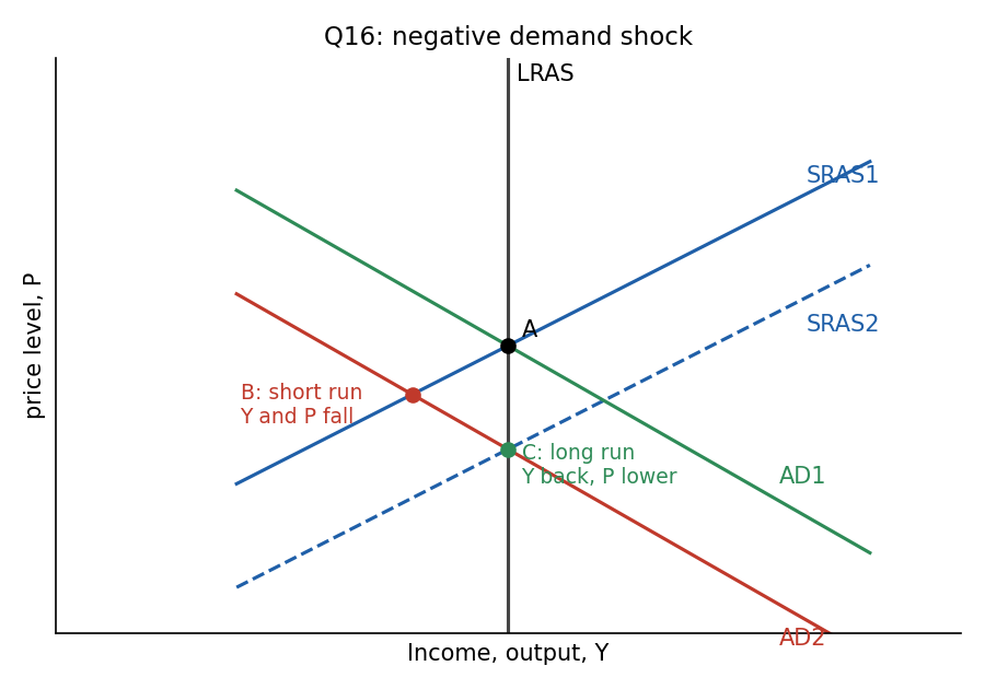
- B: expectations adjust down (since ), not up. Upward revision would shift SRAS left.
- C: prices fall in the short run when SRAS is upward-sloping. Unchanged prices is the fixed-price (Keynesian cross) case.
- D: output moves in the short run, and prices end lower in the long run.
🗣️ In plain EnglishWeak demand pushes output and prices down. Over time everyone expects lower prices, costs fall, and the economy recovers at a lower price level.
Q17 — AK model: saving rate for permanent growth
Question. Production function . The break-even investment rate is 10%. If the government can indirectly set the saving rate, what should the target be to induce permanent growth of income?
- A. Above 20%
- B. Less than 20%
- C. Exactly 20%
- D. Between 10% and 30%
Answer: A
with is the AK (endogenous growth) model: constant returns to capital. Growth of capital is
Permanent growth needs , so . Since , income grows at the same rate.
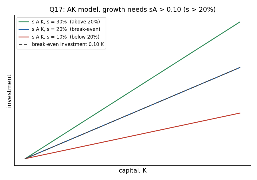
Investment must lie above the break-even line .
- B (below 20%): investment is below break-even, so capital and income shrink.
- C (exactly 20%): investment equals break-even, so zero growth. Growth is flat, not positive.
- D (10% to 30%): includes values from 10% to 20% where income shrinks, so it does not guarantee growth.
🗣️ In plain EnglishWith no diminishing returns, saving feeds permanent growth, but only if you save more than 20%. At exactly 20% you just stand still.
Q18 — Growth rate of real balances
Question. . Money supply grows 5%, real output grows 3%, velocity rises 1%. What is the growth rate of real balances?
- A. 2 percent
- B. 3 percent
- C. 5 percent
- D. 4 percent
Answer: A
Real balances , so in growth rates: .
Cross-check with the quantity equation : , then real balances grow . See Velocity of Money, Money Demand.
- B (3): that is inflation, or real output growth.
- C (5): that is nominal money growth.
- D (4): , adds velocity growth instead of subtracting it.
🗣️ In plain EnglishReal money balances grow like output but shrink when velocity speeds up: 3% minus 1% is 2%.
Q19 — Necessary condition for money neutrality
Question. Which is a necessary economic condition for money neutrality?
- A. Supply-side determined equilibrium
- B. Demand-side determined equilibrium
- C. Fixed government expenditure
- D. Fixed inflation expectations
Answer: A
Money Neutrality says changes in move only nominal variables. That requires output to be determined by the supply side (labour, capital, technology), so it does not respond to demand-side money changes.
- B: if output were demand-determined, a money change could move , which breaks neutrality.
- C: neutrality is about money, not fiscal policy. need not be fixed.
- D: expectations are not fixed. Under neutrality they adjust and move the nominal rate one-for-one (Fisher Effect).
🗣️ In plain EnglishMoney can only be neutral if real output is set by supply factors like workers and technology, not by how much people spend.
Q20 — Liquidity preference: excess money supply
Question. Short-run theory of liquidity preference. If the demand for real money balances is lower than the supply, individuals will
- A. purchase interest-earning assets so the interest rate would fall
- B. sell interest-earning assets so the interest rate would rise
- C. sell interest-earning assets so the interest rate would fall
- D. purchase interest-earning assets so the interest rate would rise
Answer: A
means people hold more cash than they want, so they buy bonds. Higher bond demand raises bond prices and lowers the interest rate, until money demand rises to equal supply. See Liquidity Preference.
- B and C: selling bonds is what people do when they have too little cash. That is the Q3 mechanism.
- D: buying bonds pushes the interest rate down, not up.
🗣️ In plain EnglishToo much cash on hand means people go buy bonds, which drives interest rates down.
Q21 — Price level rises under a fixed exchange rate
Question. Mundell-Fleming with a fixed exchange rate. If the price level rises, the central bank will
- A. buy foreign currency
- B. sell foreign currency
- C. not intervene in the foreign exchange market
- D. buy domestic currency
Answer: A
Higher lowers , so LM* shifts left, which would push the exchange rate up (appreciation) above the peg. To hold the peg the central bank must sell domestic currency and buy foreign currency. That increases and shifts LM* back right. See Fixed Exchange Rate.
- B and D (sell foreign / buy domestic currency): these two are the same action. They shrink , pushing LM* further left and appreciating the currency even more.
- C: not intervening would let the currency leave the peg, which a fixed regime rules out.
🗣️ In plain EnglishIf prices rise and the currency starts to strengthen past the peg, the central bank sells its own currency (buying foreign money) to hold the rate steady.
Q22 — Why the AS curve is bow-shaped
Question. The AS is normally bow-shaped, because
- A. when output is lower than normal, it is less costly to boost production relative to when output is higher than normal
- B. when output is lower than normal, it is more costly to boost production relative to when output is higher than normal
- C. when output is lower than normal, it is as costly to boost production as when output is higher than normal
- D. the fraction of fixed-price firms decreases when output level increases
Answer: A
In a slump there is idle capital and labour, so output can rise cheaply without big price increases and the curve is flat. Near full capacity, expansion requires bidding up wages and input prices, so the curve gets steep. (Lecture: Reagan's 1982 tax cuts hit the flat part, output rose and inflation barely moved.) See Short-Run Aggregate Supply, SRAS Curve.
- B: reversed.
- C: equal costs at all levels is the straight-line SRAS, not a bow.
- D: sounds like a sticky-price mechanism, but in the lecture's Sticky-Price Model the fixed-price share is a given parameter. The lecture's explanation of the bow shape is capacity and idle resources.
🗣️ In plain EnglishWhen the economy has spare capacity, firms can produce more cheaply. When it's already stretched, extra output costs much more, so prices jump.
Q23 — The long-run Phillips curve
Question. In the long run, Phillips' curve
- A. is vertical
- B. is horizontal
- C. has negative slope
- D. has positive slope
Answer: A
In the long run , so reduces to , giving for any inflation rate. The curve is vertical at the natural rate (Natural Rate of Unemployment, Natural-Rate Hypothesis).
- B: horizontal would mean inflation is fixed while unemployment varies freely.
- C: negative slope is the short-run Phillips curve.
- D: positive slope would mean higher inflation brings more unemployment, which neither run predicts (outside supply-shock episodes).
See Phillips Curve.
🗣️ In plain EnglishIn the long run people's inflation expectations catch up, so you can't trade inflation for lower unemployment. Unemployment sits at its natural rate no matter the inflation.
Q24 — Short-run monetary expansion
Question. Monetary expansion in the short run ________ the ________ interest rate
- A. lowers, real and nominal
- B. lowers, real but not the nominal
- C. rises, real and nominal
- D. rises, real but not the nominal
Answer: A
with fixed means , so LM shifts right and falls. In the short run expected inflation is unchanged, so the Fisher equation means the nominal rate falls by the same amount. See Fisher Effect, Nominal Interest Rate, Real Interest Rate.
- B: would need to rise one-for-one with the cut, which happens in the long run, not the short run.
- C and D: rates rise only with a contractionary move.
🗣️ In plain EnglishMore money in the short run means cheaper borrowing. Because expected inflation hasn't moved yet, both the real and nominal rates fall.
Q25 — A fall in the world interest rate (floating M-F)
Question. Mundell-Fleming with a floating exchange rate: a fall in the world interest rate will
- A. raise investments, but lower net exports in a greater magnitude
- B. raise investments, but lower net exports in a lower magnitude
- C. raise investments, but lower net exports at the same magnitude
- D. lower investments, but increase net exports in a lower magnitude
Answer: A
Small open economy, so falls.
- rises (cheaper borrowing), which shifts IS* right.
- Lower raises money demand at a given , so LM* shifts left: equilibrium falls.
- The currency appreciates (higher ), so NX falls.
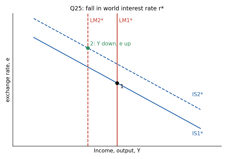
Using with (so too) and , net exports must fall by more than rises: , and both terms are negative.
- B: ignores that falls overall, so NX falling by less than the rise in would need to rise.
- C: equal magnitudes would leave (and ) unchanged, which contradicts the LM* shift.
- D: investment rises when borrowing gets cheaper.
🗣️ In plain EnglishCheaper world interest rates boost investment, but they also make the currency strong and shrink output, so the drop in net exports outweighs the rise in investment.
One-page recap
| Q | Topic | Answer | Source |
|---|---|---|---|
| 1 | Tax on saving, golden rule | A (income per person falls) | AI-solved |
| 2 | IS-LM numbers | A (, ) | Official |
| 3 | transition | A (sell bonds, up) | Official |
| 4 | M-F floating, tax cut | A (point B, appreciation) | Official |
| 5 | Large open economy, | A ( falls, NX falls) | Official |
| 6 | Sacrifice ratio and Okun | A (4; 8) | Official |
| 7 | Cost-push, long run | A (back to A) | Official |
| 8 | Solow returns to capital | A (decreasing, fixed) | AI-solved (low confidence) |
| 9 | Balanced-budget multiplier | A ($0.2B; $1B) | Official |
| 10 | Import quota, floating | E (first option) | Official |
| 11 | Higher consumption share | A ( rises) | Official |
| 12 | Bond-financed | C ( unchanged) | Official |
| 13 | Money now vs announced | A (neutral in both) | Official |
| 14 | MPK/APK | A (consumption maximized) | AI-solved |
| 15 | Steady-state | A (2.5) | AI-solved |
| 16 | Negative demand shock | A | Official |
| 17 | AK saving threshold | A (above 20%) | Official |
| 18 | Real balance growth | A (2%) | Official |
| 19 | Condition for neutrality | A (supply-side) | Official |
| 20 | Excess money supply | A (buy bonds, falls) | Official |
| 21 | Fixed rate, rises | A (buy foreign currency) | Official |
| 22 | Bow-shaped AS | A (cheaper when slack) | Official |
| 23 | Long-run Phillips curve | A (vertical) | Official |
| 24 | Short-run monetary expansion | A (real and nominal fall) | Official |
| 25 | Fall in | A (NX falls by more) | Official |
Every key answer is the first optionIn the official key all 21 answers are option A (Q10's "E" is also the first option). Papers are shuffled per student, so this is probably the version-0 (Tofes 0) layout. My four AI-solved answers also come out as A by working, not by pattern.
Related Notes
Macro-Economics II · Lec_03-Classical Theory & National Income · Lec_04-The Monetary System · Lec_05-Inflation · Lec_06-AS-AD Model & Economic Fluctuations · Lec_07-Aggregate Demand I & the IS-LM Model · Lec_08-Aggregate Demand II & Applying the IS-LM Model · Lec_09-The Open Economy Revisited & Mundell-Fleming Model · Lec_14-Aggregate Supply & the Phillips Curve