
Macro II 3058 — Moed A, 19 July 2021 (online version)
- #macro-economics-ii
- #past-paper
- #worked-solution
- #solow
- #is-lm
- #mundell-fleming
- #phillips-curve
- #hysteresis
Macro II 3058 — Moed A, 19 July 2021
Part of: Macro-Economics II Moed A, 19 July 2021 — Macroeconomics II (3058), Dr. Alon Cohen, 25 multiple-choice questions, 4% each, open books Builds on: Lec_03-Classical Theory & National Income, Lec_05-Inflation, Lec_06-AS-AD Model & Economic Fluctuations, Lec_07-Aggregate Demand I & the IS-LM Model, Lec_08-Aggregate Demand II & Applying the IS-LM Model, Lec_09-The Open Economy Revisited & Mundell-Fleming Model, Lec_14-Aggregate Supply & the Phillips Curve
Which answers are AI-writtenThe source has only a partial key: about 8 questions carry a "(correct)" marker, and those markers belong to a sibling version of the paper in which one word was swapped (see the note on the key below). Everything else has no key.
- Partial key, checked against the paper as printed: Q5, Q6, Q8, Q11, Q13, Q17, Q19, Q21.
- AI-solved, no key (Alfie's decision, 2026-11-20): Q1, Q2, Q3, Q4, Q7, Q9, Q10, Q12, Q14, Q15, Q16, Q18, Q20, Q22, Q23, Q24, Q25. Each carries its own warning callout. Where a sibling-version note exists it was used only as a cross-check.
- Solow growth (Q1 to Q6) has no lecture deck in the vault. Those answers rest on the standard Solow model, not on the notes.
How the source key worksThe source file is an "online version" of the Tofes 0 paper. Highlighted words in each question mark where the wording differs from a sibling version, and a line starting with
*gives the sibling's original word and its answer letter (for example "income: b" under Q1, where the sibling asked about income per worker). The sibling answers are not the answers to this paper's wording, but they let me check my own working: in every case my result is the mirror or the variant of the sibling answer.
What this paper tests
- Q1 to Q6: Solow growth. Steady state from , golden rule, population growth with a fixed factor, and what "sustained growth" needs (technology, or constant returns to capital).
- Q7 to Q9, Q24, Q25: AD-AS and supply. Fixed-price vs flexible-price AS, stabilising a demand shock, reading shifts on a graph, and the sticky-price model.
- Q10 to Q17: Keynesian cross and IS-LM. Multipliers, solving IS and LM numerically, liquidity preference, and policy under different central-bank rules.
- Q18 to Q21: Mundell-Fleming. Fixed vs floating, risk premium, and price-level changes.
- Q22, Q23: Phillips curve. Hysteresis in the natural rate, and the cost of disinflation via Okun's law.
Intuition: the rule for "which shift moves what"Almost every graph question reduces to two steps: (1) which curve shifts, and which way? (2) read the new intersection. Do not try to recall the answer; redraw the two curves in 10 seconds.
Q1 — Steady-state consumption per worker
, depreciation , saving rate , no population growth, no technology. What is steady-state consumption per worker?
- A. 1.36
- B. 2
- C. 8
- D. 0.68
AI-written answer, not official. Check before relying on it.Solow growth is not covered by a lecture deck. The sibling version of this question asked for income per worker (answer letter b, value 2), which matches the intermediate step below.
Answer: A. 1.36
Per worker, . In steady state, investment per worker equals depreciation:
Why the others are wrong
- B (2) is steady-state income per worker . It forgets that consumption is only the share of income.
- C (8) is the capital stock per worker .
- D (0.68) is the consumption share , not the level.
🗣️ In plain EnglishIn the long run the economy settles where the new capital people save each year ( of output) just replaces the capital that wears out ( of the stock). That happens at , which produces . People eat the they do not save, so .
Q2 — Moving to the golden rule by raising the investment rate
"Consumption is proportional to income per worker. Therefore, when moving towards the golden-rule steady state by increasing the investment rate, income per worker continuously rises and thus consumption continuously rises as well. True or false?"
- A. False. Income per worker indeed continuously rises, but consumption falls and then rises.
- B. False. Income per worker indeed continuously rises, but consumption rises and then falls.
- C. False. Income per worker continuously falls, consumption rises and then falls.
- D. True.
AI-written answer, not official. Check before relying on it.Not covered by a lecture deck. The sibling version said "decreasing" and its answer letter was c, which is the mirror image of the answer below.
Answer: A
Raising (we start below the golden rule, otherwise nobody would raise it) works in two stages:
- On impact, consumption is and has not moved yet, so a higher makes consumption fall immediately.
- Over time, higher investment builds the capital stock, so rises every period. Consumption climbs back and ends above its old level, because the golden-rule maximises steady-state .
So income rises continuously, while consumption falls and then rises.
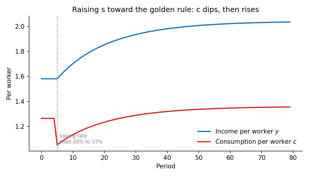
Illustrative simulation using Q1's technology (, ): jumps from 20% to the golden-rule value . Income climbs steadily; consumption drops on impact, then recovers above its starting level. The paths are for shape only; the paper gives no numbers for this question.
Why the others are wrong
- B gets the shape backwards (consumption does not rise first). It describes the opposite journey, from above the golden rule down to it.
- C has income falling, which is what happens only when is cut. The question says "increasing".
- D is the tempting trap: consumption is , so the "proportional" claim holds only for a fixed .
🗣️ In plain EnglishSaving more means you eat less today so you can have more machines tomorrow. Consumption therefore dips first and only later rises above where it started. Income just keeps rising as machines pile up.
Q3 — Land as a third input
An economy with capital, labour and fixed land, so the production function shows decreasing returns to scale in and . If labour grows at , then in the steady state, income per worker ______ and total income ______.
- A. decreases; total income increases
- B. increases; total income increases
- C. is unchanged; total income is unchanged
- D. is unchanged; total income increases
AI-written answer, not official. Check before relying on it.Not covered by a lecture deck. The sibling version (capital and labour only, constant returns) had answer letter d, which is the CRS benchmark I use below.
Answer: A. decreases; total income increases
Benchmark (constant returns): with CRS, settles at a constant, so is constant and grows at . That is option D, the sibling's answer.
With a fixed factor: write with . Land is fixed, so more workers share the same land, and per-worker output is pulled down. Per worker,
Substituting gives , which falls as grows because . Total income still rises because .
Why the others are wrong
- B ignores the land constraint (more workers on the same land cannot raise output per worker).
- C is wrong on both counts: total income still rises with more workers.
- D is the answer only under constant returns, where nothing is fixed.
🗣️ In plain EnglishMore workers on the same plot of land means each person gets less to work with, so income per person falls. But more people still produce more in total, so total income rises.
Q4 — Growth of output per effective worker
In a Solow model with technological change, population grows at 2% and the efficiency of labour grows at 3%. In the steady state, output per effective worker grows at ______ percent.
- A. 0
- B. 2
- C. 3
- D. 5
AI-written answer, not official. Check before relying on it.Not covered by a lecture deck. The sibling asked about output per worker (answer letter c, which is 3%), consistent with the table below.
Answer: A. 0
"Steady state" in this model means per-effective-worker variables (, ) are constant. The table shows each growth rate:
| Variable | Steady-state growth |
|---|---|
| Output per effective worker | 0 |
| Output per worker | |
| Total output |
Why the others are wrong
- B (2) is the population growth rate , irrelevant once we divide by .
- C (3) is the growth of output per worker (the sibling question), not per effective worker.
- D (5) is the growth of total output.
🗣️ In plain English"Per effective worker" divides out both population and technology, so the thing is constant in the long run. Growth shows up in the other ways of counting: per worker grows at , and the whole economy at .
Q5 — Factor prices when labour efficiency grows
In the Solow model with technological progress, by increasing the efficiency of labour at rate :
- A. the real wage grows at rate but the real rental price of capital is constant
- B. the real wage and the real rental price of capital both grow at rate
- C. the real wage is constant but the real rental price of capital grows at rate
- D. both the real wage and the real rental price of capital are constant
Answer: A (partial key: "marginal product of labor increases over time whereas marginal product of capital is constant")
Factor prices equal marginal products. In steady state is constant, so the marginal product of capital () is constant: the rental rate is constant. The marginal product of labour is , which grows with : the real wage grows at .
Why the others are wrong
- B has the rental price growing. That is the sibling key's "Answer b", explicitly marked as the wrong option there: capital's marginal product does not grow with .
- C reverses the two factors.
- D leaves wages flat despite rising labour productivity.
🗣️ In plain EnglishWhen each worker gets more productive, workers get paid more, so the wage rises at . Machines are no more productive than before (they are just working alongside better workers), so the rental price of capital stays flat.
Q6 — When can investment underlie sustainable growth?
- A. If capital's definition includes both physical and human resources, such that the return to capital is constant
- B. If the return to capital is diminishing, yet the technology exogenously progresses
- C. When a fraction of the labour force creates new knowledge in universities, yet this knowledge is not part of the overall definition of capital
- D. All answers are correct
Answer: A (partial key: "if the return to capital is constant")
Investment can sustain growth only if it does not run into diminishing returns. That is the endogenous-growth ("AK") logic: with a broad capital measure, the marginal product of capital does not fall as capital accumulates, so saving keeps raising growth.
Why the others are wrong
- B: growth is sustained here by technology, not by investment. With diminishing returns to capital, investment only affects the level of income.
- C: knowledge creation by a share of workers is a separate engine (research), explicitly not capital, so it is not growth underlain by investment in the sense asked.
- D is false because B and C are not correct.
🗣️ In plain EnglishMore machines usually give less and less extra output, so growth fades. Growth from investment only lasts if the payoff to investing never shrinks, as when "capital" is defined widely enough (including skills) that it never runs dry.
Q7 — What the two AS curves reflect
The vertical aggregate supply curve in the long run reflects ______; the horizontal aggregate supply curve in the short run reflects ______.
- A. the classical dichotomy; price rigidity
- B. price rigidity; the classical dichotomy
- C. the classical dichotomy; the classical dichotomy
- D. price rigidity; price rigidity
AI-written answer, not official. Check before relying on it.The sibling version swapped "short run" and "long run" (answer letter b). Here the order is the natural one.
Answer: A
In the long run prices are flexible, so output is fixed by factors and technology and nominal variables (money, prices) do not affect real ones: the classical dichotomy (Lec_05-Inflation) gives a vertical curve at . In the short run prices are rigid, so firms meet demand at the posted price: the horizontal curve (Lec_06-AS-AD Model & Economic Fluctuations).
Why the others are wrong: B swaps the two; C credits the dichotomy for short-run flatness (the dichotomy is about flexible prices); D credits price rigidity for the long-run vertical curve (it is the opposite assumption).
🗣️ In plain EnglishLong run: prices fully adjust, so demand cannot change real output and the curve is vertical. Short run: prices are stuck, so firms just sell whatever is demanded and the curve is flat.
Q8 — Stabilising an investment slump with money
In the AD-AS model with fixed prices, firms lower investment out of pessimism. To keep unemployment at its normal rate at all times, the central bank should ______ the quantity of money. To keep the price level fixed, it should ______ the quantity of money.
- A. increase; increase
- B. increase; not change
- C. not change; increase
- D. not change; not change
Answer: A. increase; increase (partial key: the sibling with optimism has "decrease, decrease"; this paper is the mirror)
Lower investment shifts IS (and so AD) left. Unemployment stays at the natural rate only if output stays at , so the bank must shift AD back right by raising (LM shifts right). The same restored AD keeps the price level from falling in the long run.
IntuitionBoth goals demand the same thing: undo the fall in aggregate demand. There is no conflict between stabilising output and stabilising prices when the shock hits demand. A supply shock is different, because there the two goals diverge (Q9, Q24).
Why the others are wrong
- B, D leave unchanged while AD is lower: the price level then falls and unemployment rises above normal.
- C sets the two goals against each other, but with a demand shock they coincide.
🗣️ In plain EnglishA gloomy slump in investment cuts demand. The central bank's fix is to print more money so demand is back where it was, which holds both unemployment and prices steady.
Q9 — Shock and return with no policy
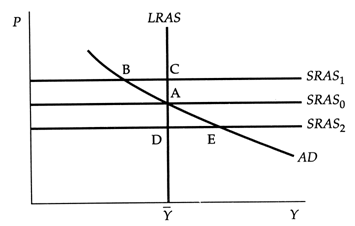
The economy is at A and is hit by a shock. It later returns to the long-run equilibrium (A) with the same price level and output, and no stabilisation policy was used. Hence:
- A. it was a shock to the supply, either negative or positive
- B. it was a positive shock to demand
- C. it was a positive shock to either demand or supply
- D. it was either a negative shock to supply or a positive shock to demand
AI-written answer, not official. Check before relying on it.The sibling version asked "after a negative supply shock, the new long-run point is: A, B, C, D" (no letter given). It supports the same logic: after a supply shock the long-run point is A.
Answer: A
- Supply shock (SRAS to SRAS or SRAS): the economy moves to B or E in the short run, and when the shock fades the SRAS curve returns to SRAS. AD is unchanged, so the long-run point is A again. This works for a negative or a positive shock.
- Demand shock: AD shifts and stays shifted. With no policy, the long-run equilibrium is on LRAS at the new price level (not A).
Why the others are wrong
- B and D include a demand shock, which permanently changes the price level.
- C wrongly adds "demand", which cannot return to A on its own.
🗣️ In plain EnglishA one-off supply hiccup fades, and everything goes back to where it started. A demand shock leaves a lasting mark on prices, so without policy you would not land back at A.
Q10 — Raising without raising taxes
Keynesian cross: planned investment , consumption , government purchases , balanced budget (). By how much should rise, without raising taxes, to reach ?
- A. 80
- B. 0
- C. 480
- D. 400
AI-written answer, not official. Check before relying on it.The sibling asked "while keeping the budget balanced" (answer letter d, 400). The two answers differ for a clear reason (taxes move vs do not), which is the point of the highlighted word.
Answer: A. 80
Equilibrium: , so and . The gap to the target is . With fixed, the government-purchases multiplier is (Lec_07-Aggregate Demand I & the IS-LM Model):
Check: .
Why the others are wrong
- B (0) assumes the economy is already at the target, but it is at 2000.
- C (480) is the new level of , not the increase.
- D (400) is the answer only if also rises by 400 (balanced-budget multiplier of 1), which the question rules out.
🗣️ In plain EnglishEach extra shekel of spending gets spent again and again (a multiplier of 5). To lift income by 400 you need only 80 more in government spending, as long as taxes stay put.
Q11 — Solving IS-LM
Closed economy: , , , , , , . In equilibrium:
- A.
- B.
- C.
- D.
Answer: A. , (partial key: the sibling with has , , which my method reproduces)
IS (goods market):
LM (money market): , so and .
Set equal: , so and .
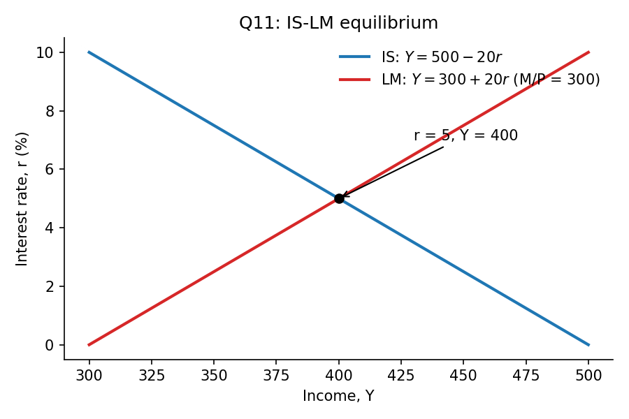
The two lines cross at , . With the LM intercept becomes 340 and the crossing moves to , , matching the sibling key.
Why the others are wrong
- B (, ) fails LM: .
- C (, ) fails IS: .
- D (, ) fails both: IS gives at and LM gives .
🗣️ In plain EnglishFind the IS line from spending equals output, the LM line from money supply equals money demand, then see where they cross: interest rate 5%, income 400.
Q12 — Excess money supply at
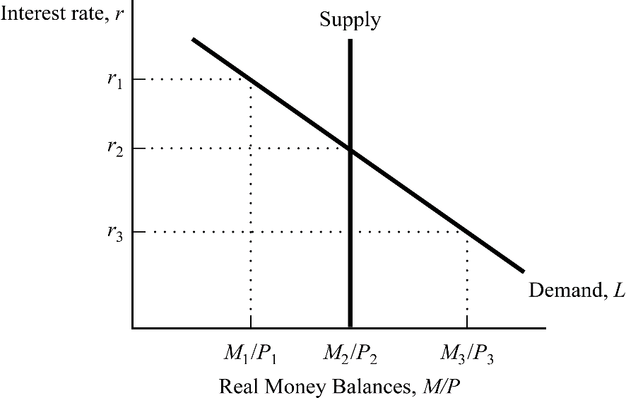
Based on the graph, if the interest rate is , then people will ______ bonds and the interest rate will ______.
- A. buy, fall
- B. buy, rise
- C. sell, fall
- D. sell, rise
AI-written answer, not official. Check before relying on it.The sibling version used (answer letter d, sell and rise). That is the mirror image of the answer below.
Answer: A. buy, fall
At the demand for money is , which is less than the fixed supply . People hold more money than they want, so they spend the excess on bonds. Higher bond demand raises bond prices, which lowers the interest rate until (money demand equals supply).
Why the others are wrong
- B has the right direction of trade but a rising rate: more bond buying pushes prices up and yields down.
- C, D describe the situation at (money demand above supply), the sibling question.
🗣️ In plain EnglishAt you are swimming in cash, so you buy bonds. Everyone buying bonds pushes bond prices up and the interest rate down.
Q13 — Does an investment fall affect the money market?
"A decrease in planned investment is a change in the markets for goods and services, thus it will not affect the equilibrium in the money market. True or false?"
- A. False. A decrease in planned investment lowers the income level which decreases the demand for money.
- B. False. A decrease in planned investment increases the interest rate which lowers the quantity demanded for money.
- C. True. The money market is not affected by changes in investment or income level.
- D. True. The money market is affected by changes in income, but not by changes in investment level.
Answer: A (partial key: "False. ... lowers the demand for money which decreases the interest rate")
Lower shifts IS left, so falls. Money demand depends on income, so the demand for money shifts left, and in the money market the interest rate falls. The two markets are linked through (Lec_07-Aggregate Demand I & the IS-LM Model).
Why the others are wrong
- B has the direction of the interest rate wrong: lower lowers .
- C denies the IS-LM link altogether.
- D concedes that income matters but then says investment cannot change income, which it can.
🗣️ In plain EnglishA fall in investment makes people poorer, so they want to hold less money. That drags the interest rate down: the goods market does leak into the money market through income.
Q14 — Tax cut on the IS-LM graph
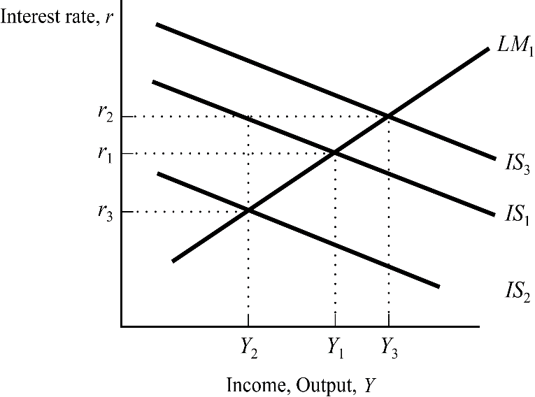
Starting from equilibrium at and , a tax cut produces which new equilibrium?
- A.
- B.
- C.
- D.
AI-written answer, not official. Check before relying on it.The sibling version said "rise" (taxes up), answer letter c, which is and is the mirror of this answer.
Answer: A.
A tax cut raises disposable income and consumption, so the IS curve shifts right (IS to IS). With LM unchanged, the new point is the intersection of IS and LM: and . Income rises, but the interest rate also rises (crowding out), so increases by less than the Keynesian-cross multiplier.
Why the others are wrong
- B and C use (to the left of ): that is IS, the shift for a tax rise.
- D pairs the lowest rate with the highest income, which no point on LM delivers.
🗣️ In plain EnglishA tax cut boosts spending, which pushes the IS curve to the right. Income goes up, and the higher demand for money pushes the interest rate up too.
Q15 — Movement along vs shift of AD
A change in income in IS-LM resulting from a change in the price level is represented by a ______ curve, while a change in income for a given price level is represented by a ______ curve.
- A. movement along the AD; shift in the AD
- B. shift in the AD; movement along the AD
- C. vertical AS; horizontal AS
- D. horizontal AS; vertical AS
AI-written answer, not official. Check before relying on it.The sibling version asked for the two blanks in the opposite order (answer letter b), consistent with the answer below.
Answer: A
The AD curve is derived from IS-LM by changing : a change in shifts LM (through ) and traces out a movement along AD (Lec_08-Aggregate Demand II & Applying the IS-LM Model). Any change at a given (a tax cut, higher ) shifts IS or LM, and so shifts AD.
Why the others are wrong: B swaps the two; C and D mention AS curves, which are not what IS-LM produces.
🗣️ In plain EnglishIf prices change, you just slide along the same AD curve. If policy or confidence changes at the same prices, the whole AD curve moves.
Q16 — Higher saving plus cheaper money management, long run
People save a larger share of income, and simultaneously a new technology lets them hold less real cash relative to income. What happens to the interest rate and output in the long run?
- A. Interest rate falls, output is unchanged
- B. Interest rate falls, the change in output is ambiguous
- C. Interest rate is unchanged, the change in output is ambiguous
- D. Interest rate increases, output is unchanged
AI-written answer, not official. Check before relying on it.The sibling asked about the short run (answer letter b, "interest rate falls, output ambiguous"). The word "long-run" here is what changes the answer to A.
Answer: A. Interest rate falls, output is unchanged
Short run (sibling answer): higher saving shifts IS left (lower , lower ). Lower money demand shifts LM right (lower , higher ). Both lower ; is ambiguous.
Long run: prices adjust until (vertical LRAS). At fixed , the IS curve alone determines : higher saving means lower demand for goods at each , so must fall to keep . The money-demand change is absorbed by the price level (money is neutral), so it does not alter or .
Why the others are wrong
- B, C carry the short-run ambiguity into the long run.
- D has the wrong sign: more saving lowers in the loanable-funds logic as well (Lec_03-Classical Theory & National Income).
🗣️ In plain EnglishIn the long run output is set by the economy's capacity, so it cannot change. Everyone saving more means more funds chasing fewer borrowers, so the interest rate falls. Cheaper money management just shows up in prices, not in output.
Q17 — Fixed money supply vs fixed interest rate after a tax cut
Alpha and Beta are identical closed economies. Both governments cut taxes by the same amount. Alpha's central bank keeps the money supply constant; Beta's keeps the interest rate constant. What happens to GDP in the new short-run equilibrium?
- A. Beta's GDP will increase more because there is no crowding out effect
- B. Beta's GDP will increase more because the IS curve shifts farther rightward under its central bank's policy
- C. Both countries' GDP will increase by the same amount
- D. Alpha's GDP will increase more because of the crowding out effect
Answer: A (partial key for the sibling with the countries swapped; the mirror gives A here)
The tax cut shifts IS right by the same amount in both countries (the shift depends on and , not on the central bank). In Alpha (fixed ) the LM curve stays put, so rises and crowds out investment: output rises by less than the full multiplier. In Beta, the bank accommodates by raising to hold fixed (a horizontal LM), so there is no crowding out and output rises by the full multiplier.
Why the others are wrong
- B is wrong on the reason: the IS shift is identical; the difference is in LM.
- C ignores that only Alpha suffers crowding out.
- D has the right mechanism (crowding out) attached to the wrong country: crowding out reduces Alpha's gain.
🗣️ In plain EnglishAlpha's higher spending pushes interest rates up, which discourages investment and eats into the gain. Beta's bank prevents the rate from rising, so Beta keeps the whole boost.
Q18 — Tax cut under a fixed exchange rate
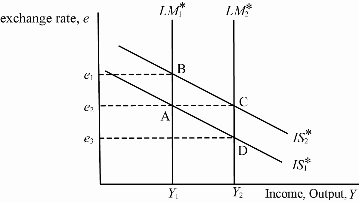
Mundell-Fleming with a fixed exchange rate; the benchmark equilibrium is A. The government cuts taxes. The new equilibrium is:
- A. C
- B. D
- C. A
- D. B
AI-written answer, not official. Check before relying on it.The sibling asked about floating rates (answer letter d, point B). The two differ exactly as theory predicts.
Answer: A. C
The tax cut shifts IS* right (IS to IS). Under floating rates, LM* stays put and the currency appreciates ( moves up to , point B: income unchanged). Under fixed rates the central bank must defend : pressure to appreciate means it buys foreign currency and sells domestic currency, increasing and shifting LM right* (LM to LM). The economy ends at C (, ): fiscal policy is fully effective.
Why the others are wrong
- B (D) is on IS: it would require LM* to shift without IS* shifting (a monetary expansion).
- C (A) ignores the tax cut.
- D (B) is the floating-rate outcome (exchange rate rises, income unchanged).
🗣️ In plain EnglishFixed rate: the central bank must hold the currency's value and ends up creating money as the tax cut pulls capital in. That extra money amplifies the tax cut, so income rises (point C). Under a floating rate the currency would just strengthen instead.
Q19 — Offsetting the income gain from a higher risk premium
"An increase in income generated by an increase in the country risk premium will not occur if there is a(n) ______ sufficient to offset the decline in the demand for money caused by the higher risk premium."
- A. decrease in the money supply
- B. increase in the money supply
- C. decrease in government spending
- D. fall in the price level
Answer: A (partial key: the marker names "currency depreciation that might boost the price of imports", which is a variant of the same mechanism)
A higher risk premium raises , which lowers money demand. Money-market balance then needs higher income: LM* shifts right, and income rises (Lec_09-The Open Economy Revisited & Mundell-Fleming Model). To stop that, we need a leftward shift in LM* of the same size, via a fall in , or a rise in (lower ), which the key's wording ("depreciation boosts import prices") describes.
Mismatch with the keyThe "(correct)" line for this question names an option that is not on this paper's list (a depreciation that raises import prices). The mechanism is the same (lower shifts LM* left); of the four printed options only A does it.
Why the others are wrong
- B shifts LM* further right and adds to the income increase.
- C shifts IS* left; it could cancel the income gain, but it does not offset the fall in money demand, which the question asks for.
- D raises , so LM* shifts further right: the opposite.
🗣️ In plain EnglishA risk premium pushes up interest rates, so people want less money. Unless the central bank mops up the extra money (cuts ), that frees demand and income rises.
Q20 — Mundell-Fleming and a falling price level
In the Mundell-Fleming model, if the price level falls, then equilibrium income
- A. rises and the real exchange rate depreciates
- B. rises and the real exchange rate appreciates
- C. falls and the real exchange rate appreciates
- D. falls and the real exchange rate depreciates
AI-written answer, not official. Check before relying on it.The sibling said "rises" (answer letter c, "falls and real exchange rate appreciates"), which is the mirror of this answer.
Answer: A
Lower raises real balances , shifting LM* right. In a floating regime, income rises and the nominal exchange rate falls (depreciation), which is what makes AD slope down in this model. The real exchange rate is . With and both falling (and fixed), falls: a real depreciation, which also lifts net exports.
Why the others are wrong
- B has the right income move but the wrong real-exchange-rate move.
- C, D have income falling, which would need a higher price level.
🗣️ In plain EnglishLower prices mean the money you hold buys more, which acts like an expansion. Income rises, the currency weakens, and our goods become cheaper abroad (real depreciation).
Q21 — Large open economy, tax rise, floating rates
A large open economy with a floating exchange rate. The government raises taxes. What happens to and net exports?
- A. Interest rate falls, net export rises
- B. Interest rate is unchanged, net export rises
- C. Interest rate is unchanged, net export is unchanged
- D. Interest rate falls, net export is unchanged
Answer: A (partial key: the sibling with a tax cut has "interest rate rises, net exports falls", and this is its mirror)
In a small open economy, and a tax rise would leave unchanged. A large economy's rate is not pinned: higher taxes shift IS* left, lowering (and in the closed-economy sense), and the lower makes the currency depreciate, which raises net exports (Lec_09-The Open Economy Revisited & Mundell-Fleming Model). The depreciation partly offsets the contraction.
Why the others are wrong
- B, C hold fixed, which is the small open economy assumption.
- C, D hold net exports fixed, but in a floating regime the depreciation always moves them.
🗣️ In plain EnglishHigher taxes cool the home economy, so the interest rate falls. A lower rate makes the currency weaker, which makes our exports more competitive.
Q22 — Hysteresis in the normal unemployment rate
The normal rate is , and the short-run Phillips curve is . The Fed wants to lower unemployment by 2 points in period 1 and then hold inflation permanently at its new level. By how much does the normal rate fall from its original level by period 4?
- A. 1.59
- B. 1.625
- C. 2
- D. 1.5
AI-written answer, not official. Check before relying on it.The sibling version's options (3.19, 3, 4, 3.25) fit a 4-point cut; , so the method below scales correctly.
Answer: A. 1.59
Measure everything as a deviation from the original normal rate , with .
- Period 1: (the planned cut). The normal rate is still . Inflation rises by point.
- Afterwards: to hold inflation at its new level, , so each period.
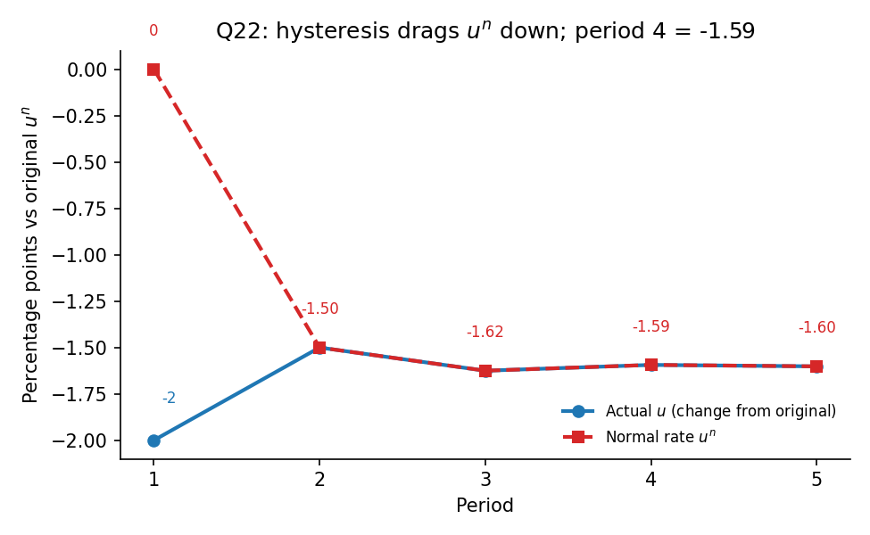
The hysteresis path computed above. The normal rate follows past actual unemployment, so it overshoots to in period 3 and settles near .
Why the others are wrong
- B (1.625) is the period-3 value.
- C (2) is the period-1 actual cut, not the normal rate.
- D (1.5) is the period-2 value.
🗣️ In plain EnglishBecause the "normal" jobless rate follows recent history, the 2-point cut slowly drags it down too. It lags the actual rate, wobbles a little, and is about 1.59 points lower by period 4.
Q23 — Cost of disinflation
The Phillips curve is and Okun's law says a 1-point change in unemployment moves GDP by 2 points. To lower inflation by 4 percentage points, the bank needs additional ____ percentage points of cyclical unemployment and a loss of ____ percentage of GDP.
- A. 8; 16
- B. 2; 4
- C. 8; 4
- D. 4; 2
AI-written answer, not official. Check before relying on it.The sibling version lowered inflation by 1 point (answer letter b, "2; 4"). The same method scales linearly to 4 points.
Answer: A. 8; 16
Set :
so cyclical unemployment is 8 points (Lec_14-Aggregate Supply & the Phillips Curve). By Okun, GDP loss points.
Why the others are wrong
- B is the answer for a 1-point cut in inflation.
- C forgets to multiply by Okun's coefficient.
- D divides instead of multiplying.
🗣️ In plain EnglishEach point of inflation you cut costs 2 points of extra unemployment and 4 points of lost output. Cutting 4 points costs 8 and 16.
Q24 — Demand-pull inflation on the graph
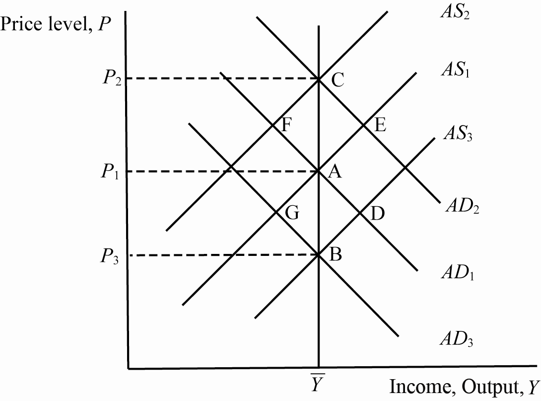
Starting from long-run equilibrium at A, a demand-pull inflation would be represented by a shift from:
- A. AD1 to AD2
- B. AD1 to AD3
- C. AS1 to AS2
- D. AS1 to AS3
AI-written answer, not official. Check before relying on it.The sibling asked about cost-push inflation (answer letter c, AS1 to AS2), which fits the identification below.
Answer: A. AD1 to AD2
Demand-pull inflation comes from higher demand: AD shifts right (AD to AD). The economy first moves to E (higher and ), then wages and expectations catch up, AS shifts up, and the economy ends at C on LRAS with a higher price level (Lec_14-Aggregate Supply & the Phillips Curve).
Why the others are wrong
- B is a demand fall (disinflation or deflation).
- C is cost-push inflation (higher input costs shift AS up).
- D is a positive supply shock (AS down), which lowers prices.
🗣️ In plain EnglishDemand-pull means too much money chasing too few goods, so the demand curve moves right. Cost-push means costs rise, so the supply curve moves up.
Q25 — High inflation and the slope of SRAS
In the sticky-price model, the higher the average inflation rate, the more frequently firms must adjust their prices. This implies that a high rate of inflation:
- A. makes the short-run aggregate supply curve steeper
- B. causes prices to be sticky
- C. should make the short-run aggregate supply curve flatter
- D. has no effect on the slope of the short-run aggregate supply curve
AI-written answer, not official. Check before relying on it.The sibling version said "low" (answer letter c, flatter), which is the mirror of this answer.
Answer: A. makes the short-run aggregate supply curve steeper
In the sticky-price model, a fraction of firms keep prices fixed. The SRAS is with (Lec_14-Aggregate Supply & the Phillips Curve). Higher average inflation means firms adjust more often, so falls, falls, and output responds less to price surprises: the SRAS curve is steeper.
Why the others are wrong
- B reverses the cause: high inflation makes prices less sticky.
- C is the low-inflation case, the sibling's answer.
- D ignores the channel through .
🗣️ In plain EnglishWhen prices are rising fast, firms reprice constantly, so fewer prices are stuck. With more flexible prices, demand changes show up in prices, not output, so the curve gets steeper.
Recap table
| Q | Topic | Answer | Source |
|---|---|---|---|
| 1 | Steady-state per worker | A (1.36) | AI-solved |
| 2 | Moving to golden rule, raising | A | AI-solved |
| 3 | Fixed land, | A | AI-solved |
| 4 | Growth per effective worker | A (0) | AI-solved |
| 5 | Wage and rental price with | A | Partial key |
| 6 | Investment and sustained growth | A | Partial key |
| 7 | Vertical vs horizontal AS | A | AI-solved |
| 8 | Money response to investment slump | A | Partial key (mirror) |
| 9 | Shock that fades with no policy | A | AI-solved |
| 10 | without tax change | A (80) | AI-solved |
| 11 | IS-LM solve | A (, ) | Partial key |
| 12 | Excess money at | A | AI-solved |
| 13 | Investment fall and money market | A | Partial key |
| 14 | Tax cut on IS-LM | A | AI-solved |
| 15 | Movement along vs shift of AD | A | AI-solved |
| 16 | Saving and money demand, long run | A | AI-solved |
| 17 | Constant vs constant | A | Partial key (mirror) |
| 18 | Fixed-rate tax cut | A (point C) | AI-solved |
| 19 | Risk premium offset | A | Partial key (mismatch noted) |
| 20 | Price level falls in M-F | A | AI-solved |
| 21 | Large open economy, tax rise | A | Partial key (mirror) |
| 22 | Hysteresis path | A (1.59) | AI-solved |
| 23 | Disinflation cost | A (8; 16) | AI-solved |
| 24 | Demand-pull on AD-AS | A | AI-solved |
| 25 | High inflation and SRAS | A | AI-solved |
Every answer is option AEvery answer I derived turned out to be the first option, which is unusual for a real exam. I checked each one by recalculation or by the mirror-image sibling answer, so I believe they are right, but it means the printed option order may differ from what was set in the real exam. Check against the original sheet if you can.
Related Notes
- Macro-Economics II
- Lec_03-Classical Theory & National Income · Lec_05-Inflation · Lec_06-AS-AD Model & Economic Fluctuations
- Lec_07-Aggregate Demand I & the IS-LM Model · Lec_08-Aggregate Demand II & Applying the IS-LM Model
- Lec_09-The Open Economy Revisited & Mundell-Fleming Model · Lec_14-Aggregate Supply & the Phillips Curve