
Moed B 2022 — Worked Solutions
- #macro-economics-ii
- #past-paper
- #worked-solution
- #multiple-choice
- #solow-growth
- #is-lm
- #mundell-fleming
- #phillips-curve
Moed B 2022 — Worked Solutions
Part of: Macro-Economics II Moed B, 21 July 2022 (Reichman University, Tiomkin School of Economics) | Macroeconomics II 3058 | Dr. Alon Cohen | 25 multiple-choice questions, 4% each, 2.5 hours, open notes, simple calculator Key concepts: Loanable Funds Market, Quantity Theory of Money, Classical Dichotomy, Keynesian Cross, Liquidity Preference, IS-LM Equilibrium, Crowding Out, Mundell-Fleming Model, Fixed Exchange Rate, Floating Exchange Rate, Country Risk Premium, Sticky-Price Model, Phillips Curve, Sacrifice Ratio Builds on: Lec_03-Classical Theory & National Income, Lec_05-Inflation, Lec_06-AS-AD Model & Economic Fluctuations, Lec_07-Aggregate Demand I & the IS-LM Model, Lec_08-Aggregate Demand II & Applying the IS-LM Model, Lec_09-The Open Economy Revisited & Mundell-Fleming Model, Lec_14-Aggregate Supply & the Phillips Curve
What this paper tests
| Questions | Topic | Lecture |
|---|---|---|
| Q1 | Classical national saving after a tax rise | Lec 03 |
| Q2, Q3, Q10 | Quantity theory, inflation, money demand | Lec 05 |
| Q4 to Q8 | Solow growth, golden rule, institutions, endogenous growth | No lecture deck (Ch 8-9) |
| Q9, Q22, Q23 | AS-AD, sticky prices, SRAS dynamics | Lec 06, Lec 14 |
| Q11 to Q14 | Keynesian cross, liquidity preference, IS-LM policy | Lec 07, Lec 08 |
| Q15 | IS-LM to the long run | Lec 08 |
| Q16 to Q21 | Mundell-Fleming, fixed and floating, risk premium, large open economy | Lec 09 |
| Q24, Q25 | Phillips curve, Okun's law, sacrifice ratio | Lec 14 |
How these answers were sourcedEvery answer below matches the official key (
Moed_B_2022_Answers.md), which covers all 25 questions, so no question here is AI-solved. The key's own explanations are terse; the "why each wrong option fails" reasoning is expanded here. Q4 to Q8 (Solow growth, institutions) have no lecture deck in this vault, so those explanations rest on the key and standard Solow results rather than on a lecture note.
Two places where the key's reasoning is thinQ3: the key's argument ("today's price level is pinned down by today's money supply") sits awkwardly with the lecture claim that a credible announcement of future money growth moves the price level today. The verdict (A) still holds, and a cleaner argument is given in Q3. Q10 quietly assumes the short-run price level P = 2 is also the long-run one.
Answer sheet
| Q | 1 | 2 | 3 | 4 | 5 | 6 | 7 | 8 | 9 | 10 | 11 | 12 | 13 |
|---|---|---|---|---|---|---|---|---|---|---|---|---|---|
| Ans | B | B | A | C | C | A | C | D | D | C | B | A | B |
| Q | 14 | 15 | 16 | 17 | 18 | 19 | 20 | 21 | 22 | 23 | 24 | 25 |
|---|---|---|---|---|---|---|---|---|---|---|---|---|
| Ans | C | D | D | A | A | B | B | D | A | C | C | C |
Q1 — Tax rise in the neoclassical model
The government raises taxes on income by $100 billion, and the neoclassical economy adjusts so that output does not change. If the marginal propensity to consume is 0.6, national saving:
- A. rises by $100 billion.
- B. rises by $60 billion.
- C. falls by $60 billion.
- D. falls by $100 billion.
Answer: B. rises by $60 billion
National saving is . Output is fixed at by the production function, and is unchanged. So only moves:
Where the other $40 billion goesDisposable income falls by $100B. Households cut consumption by $60B and cut their own private saving by T - G+100 - 40 = +60$.
Why the wrong options fail
- A (+100) treats the whole tax rise as new saving, forgetting that households pay part of it out of what they would have saved.
- C (-60), D (-100) get the sign wrong. Higher lowers and leaves alone, so cannot fall.
🗣️ In plain EnglishOutput is stuck, so a tax rise can only shift who spends. People cut spending by 60% of the lost income, and the rest of the squeeze comes out of their own saving. The government gains $100B, so national saving is up by $60B overall.
Q2 — Inflation from money demand
Money demand is , where is a constant. Money supply grows at 10%, real output grows at 3%, is constant. What is the average inflation rate?
- A. 3 percent
- B. 7 percent
- C. 10 percent
- D. 13 percent
Answer: B. 7 percent
In equilibrium . Taking growth rates with constant:
Why the wrong options fail
- A (3%) is just output growth, not inflation.
- C (10%) would be right only if output did not grow. Real balances demanded rise with , so part of the extra money is absorbed without raising prices.
- D (13%) adds instead of subtracting it.
🗣️ In plain EnglishMoney grows 10%, but a growing economy soaks up 3% of that just by needing more cash for more transactions. Only the leftover 7% chases goods and shows up as inflation.
Q3 — Lowering inflation today: Option A or B
The money-market equilibrium in growth terms is , with . The central bank wants to lower inflation today by 2% and considers:
- Option A: lower money growth by 2% today.
- Option B: lower money growth by 2% a year from now, and declare it credibly today.
Prices are fully flexible, output is fixed, and the classical dichotomy holds. Which option achieves the goal?
- A. Only option A
- B. Only option B
- C. Both options
- D. None of them
Answer: A. Only option A
Rearrange the equilibrium condition. Fixed output means is unchanged, so:
- Option A. falls by 2 today and nothing else moves, so falls by exactly 2 today. The goal is met.
- Option B. is unchanged today. The credible announcement lowers expected future inflation, which by the Fisher effect lowers the nominal interest rate and so makes negative. That changes today only through . The fall in expected inflation is at most the 2% cut, and , so inflation today falls by less than 2%. The goal is not met.
A subtlety the key glosses overThe key says B fails because "today's price level is pinned down by today's money supply". The lecture (Lec_05-Inflation) says something slightly different: a credible announcement of future money changes expected inflation and so moves the price level now. The two fit together only through the argument above: the announcement does something today, but not the full 2 points. The verdict (A) is the same either way.
Why the wrong options fail
- B assumes an announcement alone delivers the full cut. With it cannot.
- C needs B to work, which it does not.
- D ignores that A directly lowers one for one.
🗣️ In plain EnglishTo cut inflation by 2 points today, slow the money printer today. A promise to slow it next year helps a little by changing expectations, but only a fraction of the 2 points (because ).
Q4 — Saving rate below the golden rule
Output per worker is , with no technological progress or population growth. If the steady-state capital level is below its golden-rule level, the saving rate is:
- A. 25 percent
- B. more than 25 percent but less than 75%
- C. less than 25 percent
- D. 75 percent
Answer: C. less than 25 percent
For with , the golden-rule saving rate is . Steady-state rises with , so a below the golden-rule level means .
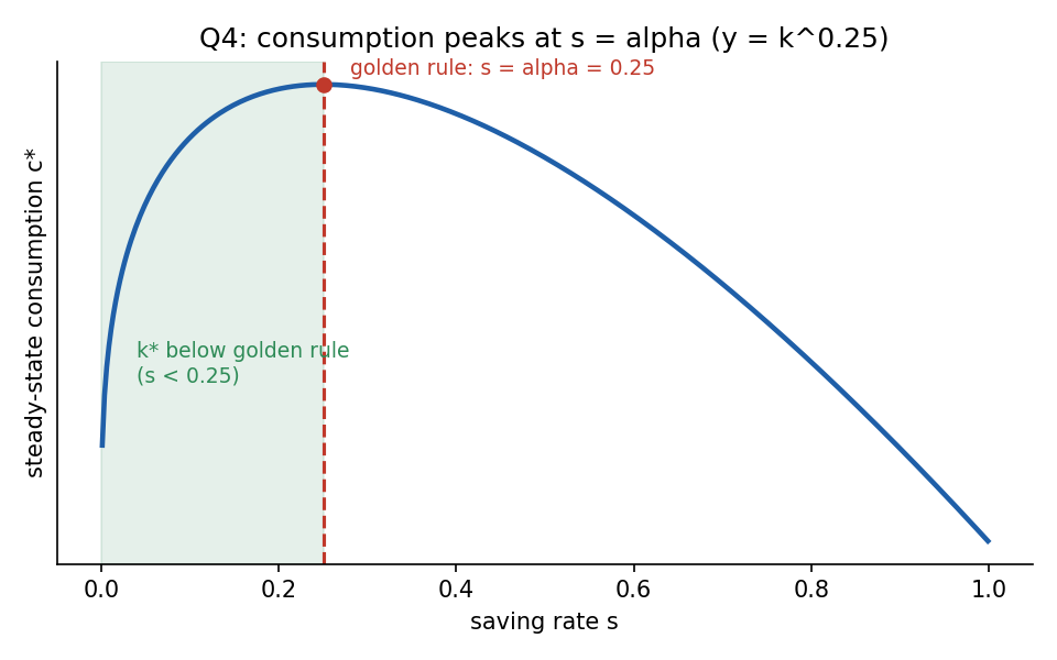
Steady-state consumption is highest at . Any saving rate to the left of that line gives a capital stock below the golden rule.
Why the wrong options fail
- A (25%) is the golden rule itself, not below it.
- B and D are above 25%, which gives more capital than the golden rule (dynamic inefficiency). The 75% figure is the capital share's complement, a distractor.
🗣️ In plain EnglishThe golden-rule saving rate here is just the capital share, 25%. If the economy has too little capital, it is saving less than that.
Not covered by a lecture deckSolow growth (Ch 8-9) has no note in this vault. The result is the standard Cobb-Douglas golden rule and matches the key.
Q5 — What does not raise steady-state output per worker
In the Solow model with population growth but no technological change, a higher steady-state output per worker can be obtained by all of the following except:
- A. increasing the saving rate.
- B. decreasing the depreciation rate.
- C. increasing the population growth rate.
- D. increasing the capital per worker ratio.
Answer: C. increasing the population growth rate
Capital accumulation is . Steady state requires .
- Higher raises the break-even line : the same capital is spread over more workers. and fall.
- Higher shifts up and lower rotates the break-even line down. Both raise and .
- Since , more capital per worker means more output per worker.
Why the wrong options fail
- A and B both raise , hence .
- D is nearly a definition: increases in . (It is not a policy lever on its own, but it is not the exception.)
🗣️ In plain EnglishMore people means the same machines are shared more thinly, so each worker produces less. Everything else on the list gives workers more capital.
Q6 — Why living standards can keep rising
In a steady state with population growth and labour-augmenting technological progress , persistent increases in living standards are possible because the:
- A. capital stock grows faster than does the labour force.
- B. capital stock grows faster than does the number of effective workers.
- C. rate of depreciation constantly decreases.
- D. saving rate constantly increases.
Answer: A. capital stock grows faster than does the labor force
| Variable | Steady-state growth rate |
|---|---|
| Labour force | |
| Effective workers | |
| Capital | |
| Capital per worker | |
| Output per worker |
grows at , faster than (growing at ). So capital per worker, and output per worker, rise at rate forever.
Why the wrong options fail
- B is false: in steady state and effective workers both grow at , which is exactly why per effective worker is constant.
- C and D are not steady-state features. and are constants, and neither can fall or rise forever.
🗣️ In plain EnglishBetter technology makes each worker count for more, so capital has to outgrow the headcount to keep up. That gap is what lifts living standards year after year.
Q7 — Institutions and climate
One explanation for greater economic development in moderate versus tropical climates is that institutions established by colonial settlers in moderate climates ______, while institutions established by colonists in tropical climates ______.
- A. were based on English common law; were based on the Napoleonic Code
- B. were based on the Napoleonic Code; were based on English common law
- C. protected property rights; were extractive and authoritarian
- D. were extractive and authoritarian; protected property rights
Answer: C. protected property rights; were extractive and authoritarian
This is the Acemoglu, Johnson and Robinson story. In moderate climates settlers meant to stay, so they built institutions that protected property rights. In tropical climates (high disease burden) colonisers did not settle and set up extractive, authoritarian regimes to take resources out.
Why the wrong options fail
- A and B are about legal origin (common versus civil law), a different literature. They also do not map neatly onto climate.
- D reverses the two climates.
🗣️ In plain EnglishWhere settlers could live safely, they built rule-of-law institutions for themselves. Where they could not, they ran extractive regimes and left. That difference still shows up in income today.
Not covered by a lecture deckInstitutions and growth have no lecture note here. The explanation follows the key.
Q8 — Saving rate and the steady-state growth rate
Assume the steady-state growth rate of income per worker is affected by the saving rate. This observation is supported:
- A. only by the Solow model.
- B. both by the Solow and by endogenous growth theory.
- C. neither by the Solow nor by endogenous growth theory.
- D. only by endogenous growth theory.
Answer: D. only by endogenous growth theory
- Solow: the steady-state growth rate of income per worker is , exogenous technological progress. The saving rate changes the level of income per worker, not its long-run growth rate.
- Endogenous growth (AK model, ): growth rate . The saving rate enters the growth rate directly.
Why the wrong options fail
- A, B wrongly credit Solow: in Solow a higher only produces a temporary growth burst on the way to a higher level.
- C ignores the AK result .
🗣️ In plain EnglishIn Solow, saving more makes you richer but not faster-growing forever. In endogenous growth, saving more keeps the growth rate itself higher.
Q9 — Supply-side determined output
If in the long run the level of output is supply-side determined, then:
- A. long-run AS is horizontal, and changes in aggregate demand affect prices but not the level of output.
- B. long-run AS is horizontal, and changes in aggregate demand affect the level of output but not prices.
- C. long-run AS is vertical, and changes in aggregate demand affect the level of output but not prices.
- D. long-run AS is vertical, and changes in aggregate demand affect prices but not the level of output.
Answer: D. long-run AS vertical; AD changes affect prices but not output
Supply-determined output means from the production function, whatever the price level. That is a vertical Long-Run Aggregate Supply curve. Shifting AD along a vertical line changes only .
Why the wrong options fail
- A and B call LRAS horizontal. A horizontal curve is the short-run, fixed-price case (see Q10).
- C has the right shape but the wrong conclusion: with a vertical LRAS, AD moves , not .
🗣️ In plain EnglishIn the long run the economy can only make so much, set by capital, labour and technology. More demand then just bids up prices.
Q10 — Money supply from the quantity equation
The long-run AS curve is vertical at and the short-run AS is horizontal at . Aggregate demand comes from the quantity theory with velocity 2. What is the quantity of money in the long run?
- A. 500
- B. 2,000
- C. 1,000
- D. 250
Answer: C. 1,000
Hidden assumptionThe question takes as the price level at the long-run equilibrium. Strictly, the horizontal SRAS at only fixes the short-run price level; the long-run is whatever clears at and could differ. The intended reading, which the key follows, is that the economy starts at the intersection, so short-run and long-run coincide.
Why the wrong options fail
- A (500) divides by twice, equivalent to using .
- B (2,000) multiplies without dividing by .
- D (250) is divided by 8, with no sensible route to it.
🗣️ In plain EnglishTotal spending is . Each unit of money is spent twice a year, so the economy needs only 1,000 units of money.
Q11 — Tax cut in the Keynesian cross
In the Keynesian-cross model, if , then a $1 billion decrease in taxes increases planned expenditure by ______ and increases equilibrium income by ______.
- A. $1 billion; $3 billion
- B. $0.75 billion; $3 billion
- C. $0.75 billion; $0.75 billion
- D. $1 billion; $1 billion
Answer: B. $0.75 billion; $3 billion
A tax cut raises disposable income by $1B, but households spend only of it, so initial planned expenditure rises by .
The tax multiplier from Lec_07-Aggregate Demand I & the IS-LM Model is:
so billion.
Why the wrong options fail
- A and D say planned expenditure rises by the full $1B, forgetting households save 25% of a tax cut.
- C stops at the first round and ignores the multiplier.
🗣️ In plain EnglishPeople spend only 75 cents of each tax-cut dollar, so the first push is $0.75B. Then that spending becomes someone's income and gets spent again, and the total builds to $3B.
Q12 — Liquidity preference
According to the theory of liquidity preference, if the demand for real money balances exceeds the supply, individuals will:
- A. sell interest-earning assets to obtain non-interest-bearing money, so the interest rate rises.
- B. sell interest-earning assets to obtain non-interest-bearing money, so the interest rate falls.
- C. purchase interest-earning assets to reduce money holdings, so the interest rate rises.
- D. purchase interest-earning assets to reduce money holdings, so the interest rate falls.
Answer: A
If people want more money than exists, they get it by selling bonds. Selling bonds pushes bond prices down, which is the same as pushing the interest rate up. This continues until money demand has fallen (higher makes holding money costlier) to equal supply.
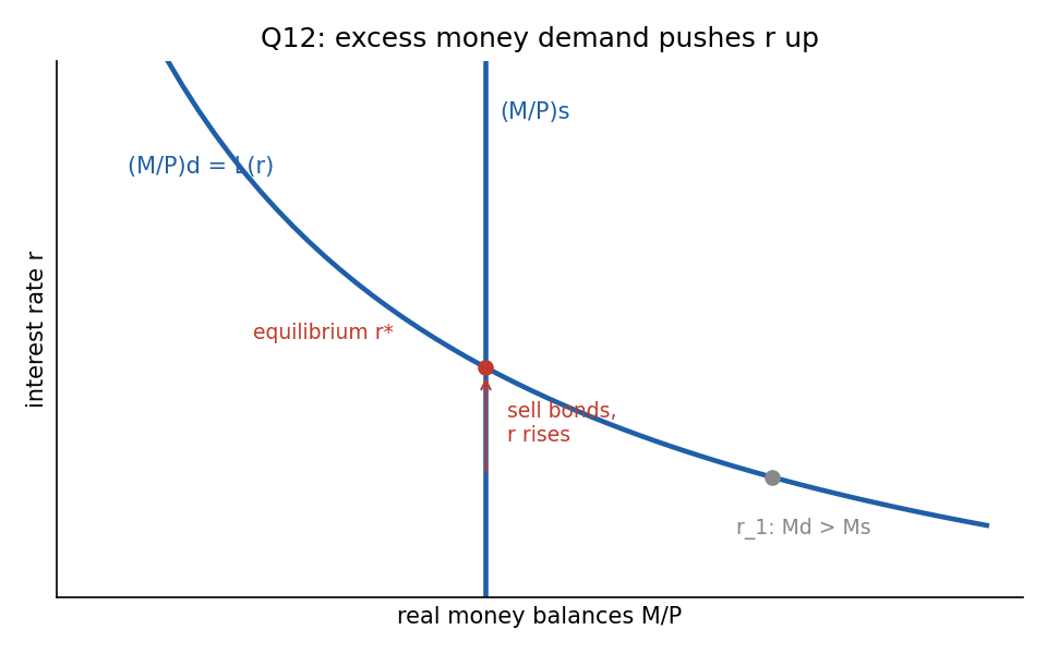
At an interest rate below equilibrium, demand exceeds the fixed real money supply. The scramble for cash drives up to the crossing point.
Why the wrong options fail
- B gets the direction wrong: selling bonds lowers their price and so raises the yield.
- C and D have people buying bonds, which is what they do when they hold too much money, the opposite case.
🗣️ In plain EnglishShort of cash? You sell bonds to get it. Lots of people selling bonds drives bond prices down, which means interest rates go up.
Q13 — A cut in G in IS-LM
Based on the graph, starting from equilibrium at interest rate and income , a decrease in government spending generates the new equilibrium:
The graph shows a single upward-sloping and three downward-sloping IS curves: (the highest), (through the initial equilibrium) and (the lowest). Dotted lines mark on the vertical axis (with highest and lowest) and on the horizontal axis (from left to right).
- A.
- B.
- C.
- D.
Answer: B.
Lower lowers planned expenditure, so shifts left from to (the lower curve). The new equilibrium is where crosses : lower income () and lower interest rate ().
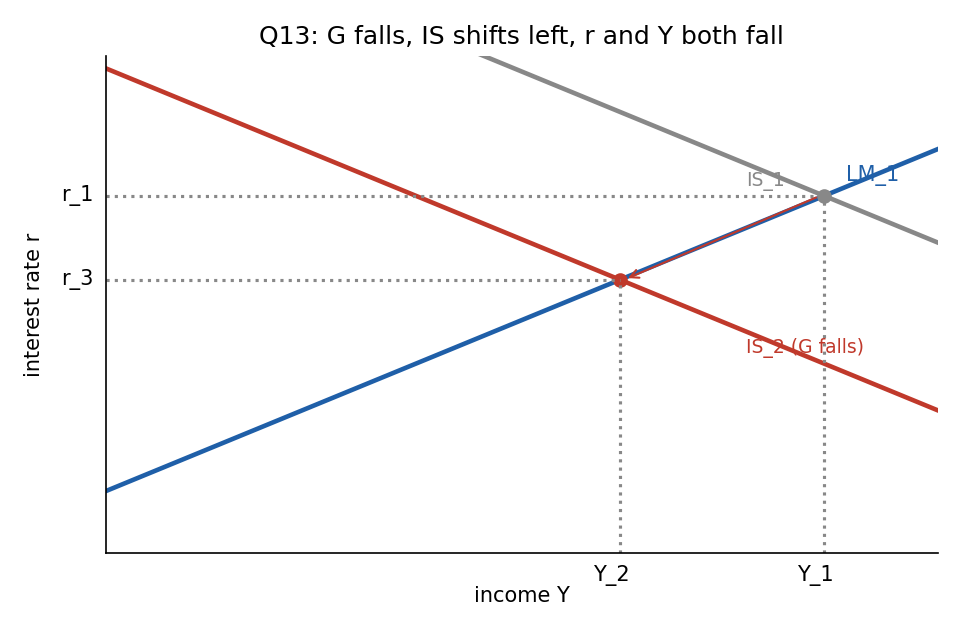
Redrawn from the exam's graph. The economy moves down along from the old equilibrium to the point at .
Why the wrong options fail
- C is the outcome on , the curve for a rise in .
- D and A pair a rate and an income that never sit together on , so no shift of IS can produce them.
🗣️ In plain EnglishLess government spending means less demand, so income drops. Lower income reduces demand for money, and the interest rate falls along with it.
Q14 — IS-LM versus Keynesian-cross multiplier
The increase in income in response to a fiscal expansion in IS-LM is:
- A. always less than in the Keynesian-cross model, regardless of the policy taken by the central bank.
- B. less than in the Keynesian-cross model unless the LM curve is vertical.
- C. less than in the Keynesian-cross model unless the central bank is committed to a fixed interest rate level.
- D. more than in the Keynesian-cross model unless the central bank is committed to a fixed income level, so that the IS curve is vertical.
Answer: C
A fiscal expansion raises income, which raises money demand and the interest rate. The higher crowds out investment (Crowding Out), so income rises by less than the Keynesian cross predicts. If the central bank pegs (an accommodating, horizontal LM), never rises, nothing is crowded out and the full multiplier is restored.
Why the wrong options fail
- A is too strong: it ignores the fixed- exception.
- B has it backwards. A vertical LM gives complete crowding out, so income does not rise at all, which is the worst case, not the exception.
- D claims IS-LM can give more than the Keynesian cross. Crowding out only reduces the multiplier, and "fixed income level" does not make IS vertical in the described way.
🗣️ In plain EnglishGovernment spending pushes interest rates up, which scares off some private investment and shrinks the boost. Unless the central bank holds rates still, you never get the full textbook multiplier.
Q15 — From the short run to the long run
If the short-run IS-LM equilibrium has income below the natural level, then in the long run the price level will ______, shifting the ______ curve to the right and returning output to the natural level.
- A. increase; IS
- B. decrease; IS
- C. increase; LM
- D. decrease; LM
Answer: D. decrease; LM
With there is slack, so prices fall. Real balances rise, which shifts LM to the right. This lowers , raises and , and continues until .
Why the wrong options fail
- A and C have prices rising, which is what happens when .
- A and B have IS shifting. Price changes work through real money balances, so they move LM, not IS.
🗣️ In plain EnglishA slump pushes prices down, which makes the money supply worth more in real terms. That lowers interest rates and pulls output back up to normal.
Q16 — Free borrowing and lending in Mundell-Fleming
In the Mundell-Fleming model, the ability to freely borrow from or lend funds abroad, for a small economy, is reflected by:
- A. a fixed level of prices, tied to the world price level
- B. the ability to export or import goods and services
- C. a vertical LM* curve
- D. a fixed interest rate, equal to the world interest rate
Answer: D
Perfect capital mobility in a small open economy forces . Any gap would trigger instant capital flows that close it (Capital Mobility).
Why the wrong options fail
- A confuses the capital account with price-level assumptions. M-F assumes sticky prices, not prices tied to the world's.
- B is about trade in goods, not borrowing and lending.
- C is a property of the money market ( with fixed), not a statement about capital mobility. It is a consequence, not the reflection.
🗣️ In plain EnglishA small country can borrow and lend as much as it likes at the world interest rate, so its own rate cannot drift away from it.
Q17 — What appreciates the exchange rate (floating)
In a small open economy with a floating exchange rate, the exchange rate appreciates if:
- A. the money supply is decreased.
- B. the money supply is increased.
- C. government spending is decreased.
- D. taxes are increased.
Answer: A
Lower shifts left. Income falls and the exchange rate rises (appreciates), since the tighter money tends to raise the interest rate and attract capital.
Why the wrong options fail
- B is the mirror image: shifts right and the currency depreciates.
- C and D shift left (lower , higher ). Under floating rates this depreciates the currency and leaves unchanged.
🗣️ In plain EnglishTightening money makes the currency more attractive to hold, so it strengthens. Cutting spending or raising taxes does the opposite.
Q18 — Monetary expansion under a fixed exchange rate
A small open economy with a fixed exchange rate is initially at equilibrium point A. After a monetary expansion, as displayed in the graph, the new equilibrium is at ____, holding everything else constant.
The graph (exchange rate against income ) shows vertical at and at , and two downward-sloping curves and . Point A is at . B is at . C is at . D is at .
- A. A
- B. B
- C. C
- D. D
Answer: A (no change)
Monetary expansion shifts right, tending towards D, where the exchange rate would fall below . To defend the peg the central bank must buy its own currency by selling foreign reserves, which shrinks the money supply and shifts back. Monetary policy cannot move or under a peg.
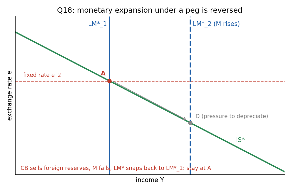
The expansion pushes the economy towards D, but defending the peg reverses it. The economy stays at A.
Why the wrong options fail
- D is where a floating economy would end up after the expansion.
- B and C both lie on , which needs a fiscal shift. C ( at ) is the outcome of a fiscal expansion under a peg, not a monetary one.
🗣️ In plain EnglishUnder a peg, the central bank has to hold the exchange rate steady, so it must undo any extra money it prints. Monetary policy just doesn't work here.
Q19 — A higher country risk premium
In the Mundell-Fleming model, if political turmoil raises the risk premium on a country's interest rate, the exchange rate will likely ______.
- A. increase
- B. decrease
- C. remain constant
- D. either increase or decrease, depending on whether the IS* or LM* curve shifts more
Answer: B. decrease (depreciate)
With a risk premium, , so a higher raises the domestic interest rate. Investors demand compensation for risk, and capital flees. Demand for the domestic currency falls and the exchange rate depreciates (Country Risk Premium). Income is the ambiguous variable, not the exchange rate.
Why the wrong options fail
- A thinks the higher interest rate attracts capital. But the extra interest is just compensation for risk, not a better return.
- C ignores the capital outflow entirely.
- D is a trap. The two curves both push down: the higher lowers investment (IS* left), while lower money demand shifts LM* right. They disagree only about , not about .
🗣️ In plain EnglishPolitical turmoil scares investors, who sell the currency and pull money out. Less demand for the currency means it weakens.
Q20 — A higher price level under floating rates
In Mundell-Fleming with flexible exchange rates, an increase in the price level results in a(n) ______ in the real exchange rate and a(n) ______ in net exports.
- A. increase; increase
- B. increase; decrease
- C. decrease; decrease
- D. decrease; increase
Answer: B. increase; decrease
Higher lowers real balances , shifting left. The exchange rate rises (appreciates). Domestic goods now cost more abroad and foreign goods cost less at home, so net exports fall. This is the negative slope of the open-economy AD curve.
Why the wrong options fail
- A pairs an appreciation with rising net exports, but a stronger currency hurts exports.
- C and D have the currency weakening, but a lower pushes the opposite way.
🗣️ In plain EnglishHigher domestic prices shrink real money, which strengthens the currency and makes our goods pricier abroad. Exports suffer and net exports fall.
Q21 — Monetary contraction in a large open economy
In a large open economy with a floating exchange rate, such as the United States, in the short run, a monetary contraction:
- A. raises the interest rate, lowers investment and income, but does not affect the exchange rate.
- B. raises the exchange rate, lowers net exports and income, but does not affect the interest rate.
- C. initially raises the exchange rate, causing arbitrageurs to sell dollars and return the money supply to its initial level.
- D. raises the interest rate and lowers investment and income, but also raises the exchange rate and lowers net exports.
Answer: D
A Large Open Economy mixes the closed-economy and small-open cases. Both channels operate:
- Closed-economy channel: less money raises , which lowers and .
- Open-economy channel: the higher draws in foreign capital, so the exchange rate rises and net exports fall.
Both channels reduce .
Why the wrong options fail
- A ignores the exchange-rate channel: a higher does attract capital.
- B forgets the interest rate does move, since the economy is large enough to affect it.
- C describes the central bank defending a peg. Under floating rates there is no such reversal.
🗣️ In plain EnglishA big economy gets both effects: tighter money pushes interest rates up (hurting investment) and strengthens the currency (hurting exports).
Q22 — The sticky-price model
According to the sticky-price model, deviations of output from the natural level are ______ deviations of the price level from the expected price level.
- A. positively associated with
- B. negatively associated with
- C. not related to
- D. equal to
Answer: A. positively associated with
The SRAS is with . When , firms with sticky prices sell more, so .
Why the wrong options fail
- B reverses the sign: surprise price rises raise output.
- C ignores the whole short-run AS relationship.
- D claims a one-for-one link. The slope is , not 1.
🗣️ In plain EnglishWhen prices come in higher than people expected, output runs above normal, because some firms have not updated their prices yet.
Q23 — What happens when P exceeds P^e
In the short run, if the price level is greater than the expected price level, then the aggregate:
- A. demand curve will shift leftward.
- B. demand curve will shift rightward.
- C. supply curve will gradually shift upward.
- D. supply curve will gradually shift downward.
Answer: C. supply curve will gradually shift upward
means : the economy is overheating. People revise upward over time, so SRAS shifts up until returns to at a higher price level.
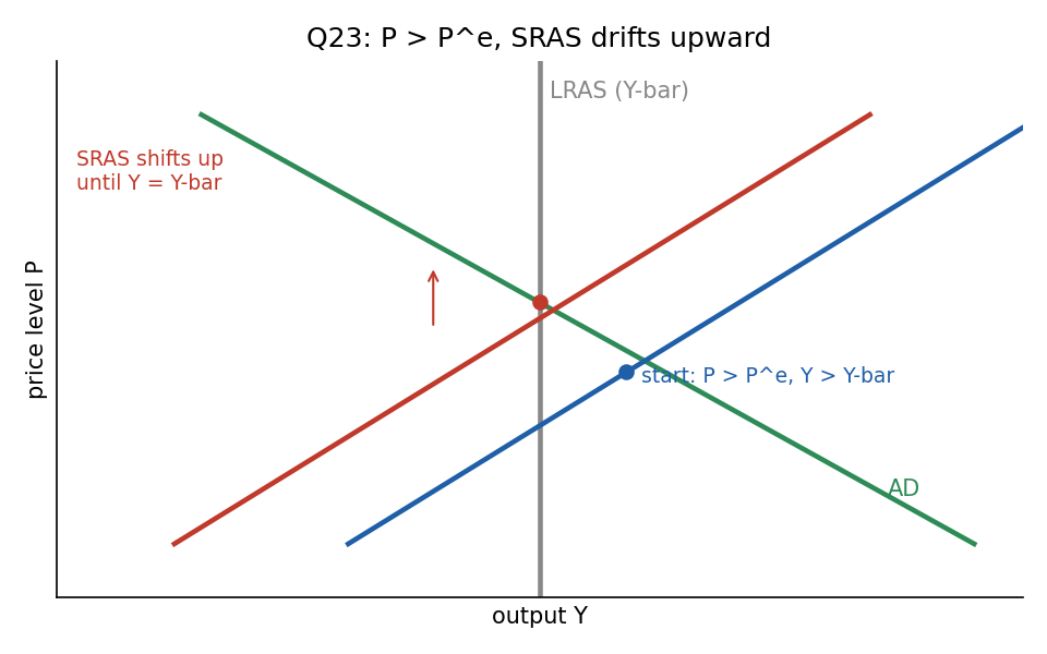
Starting with and , the blue SRAS drifts up to the red curve, which crosses AD at the natural level.
Why the wrong options fail
- A and B shift AD, but nothing in the story is a demand shift. The adjustment comes through expectations on the supply side.
- D has SRAS drifting down, which happens when (a slump).
🗣️ In plain EnglishAn overheating economy gradually raises everyone's price expectations, which shifts the supply curve up until output cools back to normal.
Q24 — The Phillips curve with low unemployment
In the long run the inflation rate is 3%. Based on the short-run Phillips curve, what is the inflation rate when unemployment is below its normal rate?
- A. 3%
- B. Less than 3%
- C. More than 3%
- D. Could be more or less than 3%
Answer: C. More than 3%
. In the long run . If then , so and .
Why the wrong options fail
- A holds only when .
- B is the case (slack).
- D is wrong because fixes the sign.
🗣️ In plain EnglishWhen jobs are unusually plentiful, wages and prices get pushed up faster, so inflation runs above its normal 3%.
Q25 — Sacrifice of output for disinflation
Okun's law says each 1% of cyclical unemployment corresponds to a 2% loss of annual GDP. The short-run Phillips curve is . If the government wants to lower inflation by 2 percentage points, how much annual GDP is lost?
- A. None, because expectations are rational
- B. 5%
- C. 10%
- D. 2%
Answer: C. 10%
Step 1: the required cyclical unemployment.
Step 2: Okun's law.
Why the wrong options fail
- A needs rational expectations and perfect credibility (Painless Disinflation). The given curve uses lagged inflation , so expectations are adaptive and the cost is real.
- B (5%) stops at the unemployment gap and forgets Okun's factor of 2.
- D (2%) is the inflation target itself, not a GDP loss.
🗣️ In plain EnglishTo get 2 points off inflation you need unemployment 5 points above normal for a year. Okun's law doubles that into a 10% hit to GDP.
Recap table
| Q | Tool | One-line answer |
|---|---|---|
| 1 | Classical saving | |
| 2 | Quantity theory | |
| 3 | Flexible prices, money demand | A: cut today. B moves by less than 2 () |
| 4 | Golden rule | , so |
| 5 | Solow with | Higher lowers and |
| 6 | Solow with | grows at against at |
| 7 | Institutions | Settlers: property rights. Tropics: extractive |
| 8 | Solow versus AK | Only AK: growth |
| 9 | AS-AD | Vertical LRAS, AD moves only |
| 10 | ||
| 11 | Tax multiplier | initial, total |
| 12 | Liquidity preference | Sell bonds, rises |
| 13 | IS-LM, falls | |
| 14 | Crowding out | Smaller than Keynesian cross, unless is pegged |
| 15 | SR to LR | falls, LM shifts right |
| 16 | M-F assumption | |
| 17 | Floating, money | falls, currency appreciates |
| 18 | Fixed rate | Stay at A |
| 19 | Risk premium | up, currency depreciates |
| 20 | AD derivation | up, up, NX down |
| 21 | Large open economy | up and up; , NX, down |
| 22 | Sticky prices | rises with |
| 23 | SRAS dynamics | , SRAS shifts up |
| 24 | Phillips curve | , so |
| 25 | Sacrifice ratio | , GDP loss |
Related notes
- Hub: Macro-Economics II
- Lec_03-Classical Theory & National Income, Lec_05-Inflation, Lec_06-AS-AD Model & Economic Fluctuations, Lec_07-Aggregate Demand I & the IS-LM Model, Lec_08-Aggregate Demand II & Applying the IS-LM Model, Lec_09-The Open Economy Revisited & Mundell-Fleming Model, Lec_14-Aggregate Supply & the Phillips Curve