
Macro II Moed A 2025 — Worked Solutions
- #macro-economics-ii
- #past-paper
- #worked-solution
- #multiple-choice
- #solow
- #classical-theory
- #is-lm
- #mundell-fleming
- #as-ad
- #phillips-curve
Macro II Moed A 2025 — Worked Solutions
Part of: Macro-Economics II Moed A, 9 February 2025 — Intermediate Macroeconomics 6827, Dr. Alon Cohen. 25 multiple-choice questions, 4% each, open notes, 2.5 hours. Builds on: Lec_03-Classical Theory & National Income · Lec_04-The Monetary System · Lec_05-Inflation · Lec_06-AS-AD Model & Economic Fluctuations · Lec_07-Aggregate Demand I & the IS-LM Model · Lec_08-Aggregate Demand II & Applying the IS-LM Model · Lec_09-The Open Economy Revisited & Mundell-Fleming Model · Lec_14-Aggregate Supply & the Phillips Curve
ALL 25 questions are AI-solved, not officialThis is a Tofes 0 paper (master version, no answer key). I solved every question independently, then compared with the tofes 0 convention that the correct answer is printed first (A). Independent solution and option A agreed on all 25 questions, so every warning below reads "consistent with the tofes 0 layout". Questions 1 to 4 (Solow, Ch 8-9) and Q2 (the AK model) are outside the lecture notes (no Solow deck exists), solved from the standard Solow model and the cheat sheet.
Course codeThis sitting is course 6827. Earlier papers in this folder (2021 to 2024) were course 3058. The question types are unchanged, but note the differences from the lecture notes: the Solow block (Q1 to Q4) and the AK model (Q2) have no lecture deck, and Q23 asks you to derive explicit IS and LM equations from general parameters rather than plug in numbers.
Figures missing from the PDFThe three diagram questions (Q4, Q21, Q25) have no image in the clean PDF. The images are in the docx copy of the same paper; the figures here are redrawn from those.
What this paper tests
The paper in one paragraphThe first block is long-run theory: Solow and the golden rule (Q1 to Q4), then the classical model (Q5 to Q12) with the quantity theory, loanable funds and the Fisher effect. Then comes the short-run Keynesian toolkit: Keynesian cross and IS-LM (Q13 to Q15, Q23, Q24), Mundell-Fleming (Q16, Q20 to Q22), and AS-AD and the Phillips curve (Q17 to Q19, Q25).
- Solow and golden rule (Q1 to Q4): the golden-rule condition is . Compare the two sides to know whether to save more or less.
- Classical theory and money (Q5 to Q12): output is fixed by supply, the interest rate clears the goods market, money only moves nominal variables, and .
- Keynesian cross and IS-LM (Q13 to Q15, Q23, Q24): multipliers, slope of LM, and when policy is potent or powerless.
- Open economy (Q16, Q20 to Q22): floating rates (exchange rate absorbs fiscal shocks) versus fixed rates (money is not controllable).
- Aggregate supply and Phillips curve (Q17 to Q19, Q25): short-run versus long-run, hysteresis, and the E to A to D adjustment path.
Every answer here is option A in the printed order.
Q1 — Steady state with MPK below depreciation
AI-written answer, consistent with the tofes 0 layout (answer printed first). Not official.Solow, Ch 8, has no lecture deck. Solved from the standard Solow model.
Question. If an economy is in a steady state with no population growth or technological change and the marginal product of capital is less than the depreciation rate:
- A. consumption per worker would be higher in a steady state with a lower saving rate.
- B. the economy is following the Golden Rule.
- C. consumption per worker would be higher in a steady state with a higher saving rate.
- D. the depreciation rate should be decreased to achieve the Golden Rule level of consumption per worker.
Answer: A (AI-solved)
With the golden-rule condition is . Here , so capital per worker is above the golden-rule level: the economy is dynamically inefficient (over-saving). Steady-state consumption is , and its slope in is . So less capital, reached by a lower saving rate, raises consumption.
- A. True. Lower lowers toward the golden rule, and rises.
- B. False. Golden rule needs (with ). Here , so it is not satisfied.
- C. False. A higher saving rate pushes even further above golden rule and lowers .
- D. False. is a technological parameter, not a policy lever. The economy reaches the Golden Rule by adjusting the saving rate, not by changing depreciation.
🗣️ In plain EnglishIf extra machines add less output than they wear out, the economy is saving too much. Saving less would leave people with more to consume in the long run.
Q2 — AK production function
AI-written answer, consistent with the tofes 0 layout (answer printed first). Not official.The AK model is outside the lecture notes (Ch 9, no deck). Solved from the standard AK derivation.
Question. If the per-worker production function is , where is a positive constant, in the steady state, a:
- A. higher saving rate leads to a higher growth rate.
- B. higher saving rate does not affect the growth rate.
- C. lower saving rate leads to a higher growth rate.
- D. lower saving rate does not affect the growth rate.
Answer: A (AI-solved)
Capital accumulation: , so
The marginal product of capital is constant (), with no diminishing returns. So capital, and hence , grows at the constant rate forever. The saving rate sets the growth rate itself, not just the level.
- A. True. .
- B. False. That is the standard Solow result (diminishing returns), where changes only the level. It fails here because there are no diminishing returns.
- C. False. Lower lowers .
- D. False. Same reason: matters for growth in the AK model.
IntuitionIn Solow, adding capital gets less and less productive, so the economy always settles. With every extra unit of capital is as productive as the last, so extra saving buys permanently faster growth.
🗣️ In plain EnglishWith there are no diminishing returns, so saving a bigger share makes the economy grow faster forever, not just richer once.
Q3 — Which rate to change to reach the golden rule
AI-written answer, consistent with the tofes 0 layout (answer printed first). Not official.Solow, Ch 8, has no lecture deck. Solved from the golden-rule condition.
Question. In the steady state: if the marginal product of capital net of depreciation equals 6 percent, the rate of output growth is 4 percent (as usual, we assume CRTS), to reach the Golden Rule level of the capital stock, the ____ rate in this economy must be _____.
- A. saving; increased.
- B. population growth; decreased
- C. saving; decreased
- D. total output growth; decreased
Answer: A (AI-solved)
Golden rule: . Under constant returns to scale, steady-state total output growth is (the 4 percent given). So .
Since falls as rises, an that is too high means is too low. The economy needs more capital, so the saving rate must increase.
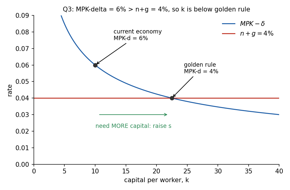
Theory diagram, curve shape illustrative: only the 6 percent and 4 percent come from the question. falls as rises, so closing the gap from 6 to 4 percent means accumulating more capital.
- A. True. Higher raises , which pushes down toward 4 percent.
- B. False. Lowering would lower the right-hand side below 4 percent, widening the gap from 6 percent. To close the gap through you would need to raise it, and population growth is not a policy tool anyway.
- C. False. A lower means even less capital and an even higher , moving away from the golden rule.
- D. False. Output growth is , not a free variable, and decreasing it widens the gap in the same way as B.
🗣️ In plain EnglishExtra capital is still paying 6% but the economy only needs to cover 4% growth, so there is too little capital. The fix is to save more.
Q4 — Reading the Solow diagram: AB/OA
AI-written answer, consistent with the tofes 0 layout (answer printed first). Not official.Solow, Ch 8, has no lecture deck. Solved from the steady-state condition, using the diagram from the docx copy.
Question. Assume no technological innovation or population growth. In this graph, when the capital-labor ratio in the steady state is OA, then the ratio AB/OA represents:
- A. the depreciation rate.
- B. the saving rate.
- C. marginal propensity to consume.
- D. marginal propensity to save.
Graph (from the docx): the curves and with a vertical line at meeting the upper curve at C and the lower curve at B.
Answer: A (AI-solved)
On the graph, is the height of the curve at , so and . In the steady state investment equals break-even investment, . With this is , so
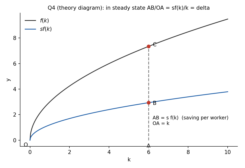
Theory diagram, shapes illustrative. is saving per worker, is , so their ratio is the depreciation rate at the steady state.
- A. True. At the steady state, saving per unit of capital exactly covers depreciation.
- B. False. The saving rate would be (the share of output saved), not .
- C. False. The MPC is the share of income consumed, which would be here; it is not .
- D. False. The MPS is the saving rate again, .
TrapWhich segment goes in the denominator decides the answer. over (output) gives ; over (capital) gives at the steady state.
🗣️ In plain EnglishThe gap is the saving, and is the capital stock. At the steady state all that saving just replaces worn-out machines, so saving per unit of capital is the depreciation rate.
Q5 — Quantity theory in the long run
AI-written answer, consistent with the tofes 0 layout (answer printed first). Not official.
Question. In the long run, according to the quantity theory of money and the classical macroeconomic theory, if velocity is constant, then ______ determines real GDP and ______ determines nominal GDP.
- A. the productive capability of the economy; the money supply
- B. the money supply; the productive capability of the economy
- C. velocity; the money supply
- D. the money supply; velocity
Answer: A (AI-solved)
Real GDP comes from the production function : supply side, the economy's productive capability (Lec_03-Classical Theory & National Income). Quantity equation: . With constant, nominal GDP moves one-for-one with the money supply (Lec_05-Inflation).
- A. True. Capability fixes ; (with constant ) fixes .
- B. False. Reversed: money cannot create real output in the long run (money neutrality).
- C. False. Velocity is held constant in the question, so it cannot determine real GDP, and it is the money supply, not velocity, that moves nominal GDP.
- D. False. Same mistake as B for the first blank, and with constant it does not "determine" anything.
🗣️ In plain EnglishIn the long run, real output depends on what the economy can produce. The money supply only decides how big the price tags are.
Q6 — What balances goods supply and demand
AI-written answer, consistent with the tofes 0 layout (answer printed first). Not official.
Question. In the classical model with fixed output, the supply and demand for goods and services are balanced by:
- A. the interest rate.
- B. taxes.
- C. fiscal policy.
- D. government spending.
Answer: A (AI-solved)
Output is fixed. Demand is . Only investment responds to the real interest rate: the rate adjusts until , which is the same as the loanable-funds market clearing (Lec_03-Classical Theory & National Income).
- A. True.
- B. False. Taxes are a policy setting, they do not adjust automatically to clear the market.
- C. False. Fiscal policy is a choice by the government. Changing it shifts the curves; it is not the clearing mechanism.
- D. False. is exogenous policy, and changes in it are balanced by changes in , not the other way round.
🗣️ In plain EnglishWhen output is fixed, the interest rate is the price that makes the amounts people want to buy match what exists to buy.
Q7 — Saving exceeds investment demand
AI-written answer, consistent with the tofes 0 layout (answer printed first). Not official.
Question. In the classic model: if saving exceeds investment demand, and consumption is not a function of the interest rate:
- A. the interest rate will fall.
- B. the demand for loans exceeds the supply of loans.
- C. the interest rate will rise.
- D. saving will fall.
Answer: A (AI-solved)
Saving is the supply of loanable funds and investment is the demand. If there is excess supply, so the interest rate falls until rises to meet .
- A. True.
- B. False. It is the reverse: the supply of loans (saving) exceeds the demand (investment).
- C. False. A surplus pushes the price (the interest rate) down, not up.
- D. False. Because consumption does not depend on , saving does not depend on : is a vertical line, so it does not fall. The adjustment happens entirely through investment rising.
🗣️ In plain EnglishMore money is being offered than wanted for loans, so the price of borrowing (the interest rate) drops.
Q8 — Government spending rises, taxes unchanged
AI-written answer, consistent with the tofes 0 layout (answer printed first). Not official.
Question. According to the model developed in Chapter 3, when government spending increases but taxes are not raised, interest rates:
- A. increase.
- B. are unchanged.
- C. decrease.
- D. can vary.
Answer: A (AI-solved)
National saving is . A higher with fixed lowers public saving and so national saving, since and are unchanged. The line shifts left, and rises to clear the loanable-funds market. Investment is crowded out (Lec_03-Classical Theory & National Income).
- A. True.
- B. False. Saving falls, so must move.
- C. False. That is the effect of a tax rise or a cut in , which raises saving.
- D. False. In the Ch 3 model the direction is determined: up.
🗣️ In plain EnglishThe government borrows more, so there is less left over for firms to borrow, and the interest rate rises. This is crowding out.
Q9 — Money demand, Fisher effect and the price level
AI-written answer, consistent with the tofes 0 layout (answer printed first). Not official.
Question. Assume that the demand for real money balance is , where is national income and is the nominal interest rate (in percent). The real interest rate is fixed at 3 percent by the investment and saving functions. The expected inflation rate equals the rate of nominal money growth. If is 1,000, is 100, and the growth rate of nominal money is 2 percent, what must and be?
- A. percent,
- B. percent,
- C. percent,
- D. percent,
Answer: A (AI-solved)
Step 1, Fisher equation. Expected inflation equals money growth, . So
Step 2, money demand.
Step 3, price level. , so .
- A. True.
- B. False. ignores that . (It does not even match : with , , which gives , so B is internally consistent with money demand but built on the wrong .)
- C. False. is right, but then , so . would need .
- D. False. needs , which only happens at , not .
🗣️ In plain EnglishWork out the nominal rate first (real rate + inflation = 5%), plug it into money demand to get real money = 100, then divide the money supply by that to find P = 1.
Q10 — Money growth and the Fisher effect
AI-written answer, consistent with the tofes 0 layout (answer printed first). Not official.
Question. In the Classic Theory, a 1 percent increase in money growth will lead to rises in:
- A. inflation of 1 percent and the nominal interest rate of 1 percent.
- B. inflation of 1 percent and the nominal interest rate of less than 1 percent.
- C. inflation of 1 percent and the nominal interest rate of more than 1 percent.
- D. both inflation and the nominal interest rate of less than 1 percent.
Answer: A (AI-solved)
Quantity theory: inflation equals money growth minus real output growth, so faster money growth passes through one for one to inflation. The Fisher effect says , and is fixed by real factors (saving and investment), so . This one-for-one pass-through is the Fisher effect (Lec_05-Inflation).
- A. True.
- B. False. rising by less than 1 would need to fall; in the classical model is unaffected by money.
- C. False. rising by more than 1 would need to rise.
- D. False. Inflation rises one for one, not less.
🗣️ In plain English1% more money growth means 1% more inflation, and lenders add that 1% to the nominal interest rate to keep their real return, so both rise one for one.
Q11 — Output rises under the quantity theory
AI-written answer, consistent with the tofes 0 layout (answer printed first). Not official.
Question. According to the quantity theory of money, if output increases, ______ real balances are required, and for fixed this means ______ .
- A. higher; lower
- B. lower; higher
- C. higher; higher
- D. lower; lower
Answer: A (AI-solved)
From we get (money demand). If rises with constant, people want higher real balances. With fixed, can only rise if falls.
- A. True.
- B. False. Real balances demanded rise with output, not fall.
- C. False. First blank right, but with fixed a higher needs a lower .
- D. False. Real balances needed do not fall when income rises.
🗣️ In plain EnglishA bigger economy needs more real money to do its trading. If the amount of money is fixed, the only way to get more real money is for prices to fall.
Q12 — A money-supply increase from long-run equilibrium
AI-written answer, consistent with the tofes 0 layout (answer printed first). Not official.
Question. Assume that a closed economy starts from long-run equilibrium. If the Federal Reserve increases the money supply, then ______ increase(s) in the short run and ______ increase(s) in the long run.
- A. output; prices
- B. prices; output
- C. output; output
- D. prices; prices
Answer: A (AI-solved)
Short run: prices are sticky, so a higher raises aggregate demand and output above (Lec_06-AS-AD Model & Economic Fluctuations, Lec_08-Aggregate Demand II & Applying the IS-LM Model). Long run: prices adjust, output returns to and the full effect lands on prices (money neutrality).
- A. True.
- B. False. Reversed: prices do not move much in the short run, and output cannot rise permanently.
- C. False. Output cannot rise in the long run; it is fixed at by supply.
- D. False. Prices are sticky in the short run, so prices alone cannot be the short-run response.
🗣️ In plain EnglishMore money boosts output at first because prices are slow to change. Eventually prices catch up and output goes back to normal.
Q13 — Keynesian cross: G for a target income
AI-written answer, consistent with the tofes 0 layout (answer printed first). Not official.
Question. Using the Keynesian-cross analysis, assume that the consumption function is given by . If planned investment is 100 and is 100, then the level of needed to make equilibrium equal 1,000 is:
- A. 260.
- B. 240.
- C. 250.
- D. 200.
Answer: A (AI-solved)
Equilibrium :
With : , so (Lec_07-Aggregate Demand I & the IS-LM Model).
- A. True.
- B. False. gives .
- C. False. gives .
- D. False. gives .
Check shortcutEach extra 10 of adds to (multiplier 2.5). From 240 (Y = 950) you need 50 more, which is 20 more of : .
🗣️ In plain EnglishWrite income = spending, collect the terms (), and solve for the government spending that makes income hit 1,000: that is 260.
Q14 — Why the LM curve slopes upward
AI-written answer, consistent with the tofes 0 layout (answer printed first). Not official.
Question. An explanation for the slope of the LM curve is that as:
- A. income rises, money demand rises, and the interest rate thus rises as well.
- B. the interest rate increases, income becomes lower.
- C. the interest rate increases, income becomes higher.
- D. income rises, money demand rises, and a lower interest rate is required.
Answer: A (AI-solved)
LM is money-market equilibrium, . Higher raises money demand. With the real money supply fixed, the interest rate must rise to bring demand back down to supply (Lec_07-Aggregate Demand I & the IS-LM Model, liquidity preference).
- A. True.
- B. False. That describes the IS curve (higher lowers investment and income), and it is not an explanation of LM's slope.
- C. False. Wrong direction for any curve in this model.
- D. False. A lower would raise money demand further; to restore equilibrium you need a higher .
🗣️ In plain EnglishWhen people earn more they want more cash. Money supply is fixed, so the price of holding cash, the interest rate, has to go up.
Q15 — Government spending versus tax cuts
AI-written answer, consistent with the tofes 0 layout (answer printed first). Not official.
Question. Based on the Keynesian model, one reason to support government spending increases over tax cuts as measures to increase output is that:
- A. the government-spending multiplier is larger than the tax multiplier.
- B. government spending increases the MPC more than tax cuts.
- C. government-spending increases do not lead to unplanned changes in inventories, but tax cuts do.
- D. an increase in government spending raises planned spending, whereas tax cuts decrease it.
Answer: A (AI-solved)
Keynesian cross multipliers (Lec_07-Aggregate Demand I & the IS-LM Model):
Since , the government-spending multiplier is larger by exactly 1: spending counts in full in the first round, while a tax cut is partly saved.
- A. True.
- B. False. The MPC is a behavioral parameter of consumers, not something either policy changes.
- C. False. Any change in planned spending away from output causes unplanned inventory changes until adjusts, whichever policy caused it.
- D. False. A tax cut raises disposable income and therefore raises planned consumption.
🗣️ In plain EnglishA dollar of government spending goes straight into demand. A dollar of tax cut is partly saved, so it does less.
Q16 — Money-supply increase under a fixed exchange rate
AI-written answer, consistent with the tofes 0 layout (answer printed first). Not official.
Question. In a small open economy with a fixed exchange rate, if the central bank tries to increase the money supply, then in the new short-run equilibrium:
- A. income remains constant.
- B. income falls.
- C. the exchange rate falls.
- D. income rises.
Answer: A (AI-solved)
The money supply shifts right, which puts downward pressure on the exchange rate. To keep the peg, the central bank must buy its own currency (sell foreign reserves), which shrinks the money supply back to where it started. returns to its original position, so income is unchanged (Lec_09-The Open Economy Revisited & Mundell-Fleming Model).
- A. True. Monetary policy is powerless under fixed rates.
- B. False. Nothing in the adjustment pushes income below its starting level.
- C. False. The exchange rate is fixed by the central bank, so it cannot fall.
- D. False. That would be the floating-rate result, which is the opposite regime.
🗣️ In plain EnglishUnder a peg, the central bank has to reverse any money it creates to defend the exchange rate, so income stays put.
Q17 — Phillips curve trade-off
AI-written answer, consistent with the tofes 0 layout (answer printed first). Not official.
Question. The Phillips curve implies that there is a negative tradeoff between inflation and unemployment:
- A. in the short run only.
- B. both the short run and long run.
- C. in the long run only.
- D. in neither the short run nor the long run.
Answer: A (AI-solved)
The short-run Phillips curve slopes down (unemployment below the natural rate comes with higher inflation). In the long run expectations catch up and the curve is vertical at the natural rate (Lec_14-Aggregate Supply & the Phillips Curve).
- A. True.
- B. False. There is no long-run trade-off (natural-rate hypothesis).
- C. False. The long-run curve is vertical, so there is no trade-off there.
- D. False. There is a short-run trade-off.
🗣️ In plain EnglishYou can buy lower unemployment with higher inflation for a while, but once people expect the inflation the benefit disappears.
Q18 — Hysteresis
AI-written answer, consistent with the tofes 0 layout (answer printed first). Not official.
Question. The hypothesis that hysteresis may play an important role in macroeconomics implies, among other things, that:
- A. the natural rate of unemployment may increase if unemployment is high for a long period of time.
- B. workers get hysterical during long depressions.
- C. hysteresis lowers the sacrifice ratio.
- D. the history of economic thought is important to macroeconomics.
Answer: A (AI-solved)
Hysteresis means the natural rate depends on past unemployment: long spells erode skills and weaken workers' attachment, so the natural rate itself rises (Lec_14-Aggregate Supply & the Phillips Curve).
- A. True.
- B. False. A pun on the word, not economics.
- C. False. Hysteresis makes disinflation more costly, which raises the sacrifice ratio (recessions leave permanent scars).
- D. False. A pun on "history", not economics.
🗣️ In plain EnglishA long slump can leave people less employable, so the normal rate of unemployment ends up higher afterwards.
Q19 — Flexible-price firms and the SRAS curve
AI-written answer, consistent with the tofes 0 layout (answer printed first). Not official.
Question. When some firms are flexible-price firms, then, along the short-run aggregate supply curve, if the level of output is less than the natural level of output, then the price level is:
- A. less than the expected price level.
- B. greater than the expected price level.
- C. equal to the natural price level.
- D. stuck at the existing price level.
Answer: A (AI-solved)
In the sticky-price model the SRAS is with . If the last term is negative, so (Lec_14-Aggregate Supply & the Phillips Curve, Lec_06-AS-AD Model & Economic Fluctuations).
- A. True.
- B. False. happens when .
- C. False. (the "natural" price) only when .
- D. False. "Stuck" is the all-firms-sticky case (horizontal SRAS); with some flexible firms the curve is upward sloping.
🗣️ In plain EnglishIf output is below normal, flexible firms cut prices, so the price level ends up below what people expected.
Q20 — A falling price level in Mundell-Fleming
AI-written answer, consistent with the tofes 0 layout (answer printed first). Not official.
Question. In the Mundell-Fleming model with flexible exchange rates, a decrease in the price level results in a(n) ______ in the real exchange rate and a(n) ______ in net exports.
- A. decrease; increase
- B. increase; decrease
- C. decrease; decrease
- D. increase; increase
Answer: A (AI-solved)
Real exchange rate . A lower domestic makes domestic goods cheaper, so decreases. Cheaper domestic goods raise net exports (Lec_09-The Open Economy Revisited & Mundell-Fleming Model). This is also the logic behind the downward-sloping AD curve in M-F.
- A. True.
- B. False. Both signs reversed.
- C. False. Right on , but cheaper goods raise exports relative to imports.
- D. False. A fall in cannot raise , which is proportional to .
TrapThe real exchange rate here is defined as (a higher value means domestic goods are more expensive). Mixing up the direction is the usual error.
🗣️ In plain EnglishWhen home prices fall, our goods become a bargain abroad, so the real exchange rate falls and net exports rise.
Q21 — A government-spending cut under floating rates
AI-written answer, consistent with the tofes 0 layout (answer printed first). Not official.The diagram was missing from the PDF; read from the docx copy.
Question. A small open economy with a floating exchange rate is initially at equilibrium C. If there is a decrease in government spending, holding everything else constant, the new equilibrium will be at ____.
- A. D
- B. A
- C. C
- D. B
Graph (from the docx): and vertical at and ; (upper) crosses them at B and C; (lower) crosses them at A and D.
Answer: A, point D (AI-solved)
Initial equilibrium C is where meets . A cut in shifts the IS* curve left from to . Under floating rates is vertical and not moved by fiscal policy, so income stays at and the exchange rate falls (depreciates): the new equilibrium is D, where meets (Lec_09-The Open Economy Revisited & Mundell-Fleming Model).
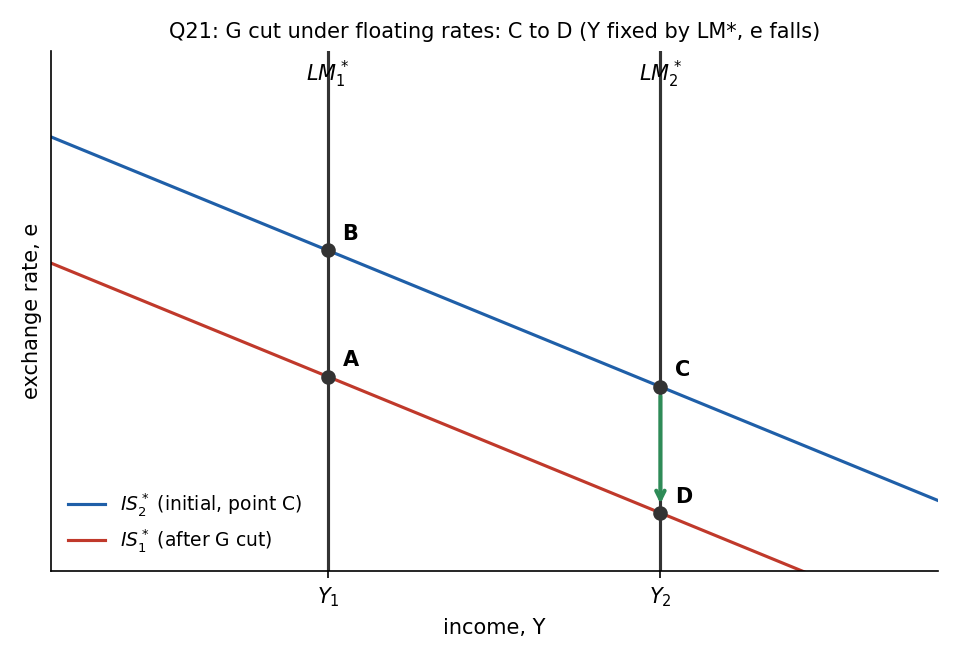
Theory diagram, shapes illustrative. The cut shifts IS left along the fixed LM*: output is unchanged, the exchange rate falls.*
- A. True. D: same , lower .
- B. False. A is on at . It would mean income falls, but under floating rates fiscal policy does not move . A is also on the lower IS*, but on the wrong LM*.
- C. False. C is the starting point, and a cut must shift IS*.
- D. False. B is on the old with , so it would require income to fall to , and no fiscal shock moves LM*.
🗣️ In plain EnglishUnder floating rates, a government spending cut doesn't change income. It just makes the currency weaker.
Q22 — Why IS* slopes down
AI-written answer, consistent with the tofes 0 layout (answer printed first). Not official.
Question. In the Mundell-Fleming model the IS* curve:
- A. slopes downward and to the right because the higher the exchange rate, the lower the level of net exports and, therefore, of short-run equilibrium income in the goods market.
- B. is vertical because there is only one investment level that is consistent with the world interest rate.
- C. is vertical because the exchange rate does not enter into the IS* equation.
- D. slopes downward and to the right because the higher the exchange rate, the higher the level of net exports and, therefore, of short-run equilibrium income in the goods market.
Answer: A (AI-solved)
IS*: . A higher makes domestic goods more expensive abroad, so falls and so does : a negative relationship, so IS* slopes down in space (Lec_09-The Open Economy Revisited & Mundell-Fleming Model).
- A. True.
- B. False. Investment is fixed by , but that does not make IS* vertical; still enters through . (It is the LM* curve that is vertical.)
- C. False. does enter through net exports.
- D. False. Slope right, but the reason has the wrong sign: a higher lowers .
🗣️ In plain EnglishA stronger currency makes our exports less competitive, so income is lower. That is why IS* slopes downward.
Q23 — When is monetary policy potent in IS-LM?
AI-written answer, consistent with the tofes 0 layout (answer printed first). Not official.Solved by deriving the equations as the question instructs.
Question. In a closed economy: if the investment demand function is and the quantity of real money demanded is , then monetary policy is relatively potent in influencing aggregate demand when is ______ and is ______ (instruction: find explicit equations for IS and LM and consider when expansionary monetary policy will lower the interest rate and raise the output the most).
- A. large; small.
- B. small; also small.
- C. small; large.
- D. large; also large.
Answer: A, large d and small f (AI-solved)
Let and let collect the autonomous terms (including , and the tax and intercept terms). Then
Setting them equal, , so
This is larger when is large and is small.
- A. True. Large : a small fall in triggers a big rise in investment (flat IS). Small : money demand barely responds to , so extra money must push down a lot (steep LM).
- B. False. A small means investment barely responds to the lower , so output barely moves.
- C. False. Both ingredients are the weak ones: small and large (the liquidity-trap direction).
- D. False. Large is good, but large lets money sit in "liquid" balances as falls, which dampens the interest-rate fall. The multiplier above shrinks as grows.
🗣️ In plain EnglishMonetary policy works best when investment reacts a lot to interest rates (large d) and money demand reacts very little (small f), so extra money pushes rates down hard and firms respond.
Q24 — IS-LM with interest-inelastic money demand
AI-written answer, consistent with the tofes 0 layout (answer printed first). Not official.
Question. Consider the IS-LM model, yet assume the demand for money is independent of the interest rate. If government spending rises by , in the IS-LM analysis, then equilibrium income rises by:
- A. zero
- B. more than zero but less than .
- C. .
- D. .
Answer: A (AI-solved)
If money demand is only, the LM curve is vertical: fixes whatever the interest rate. A fiscal expansion shifts IS right, but equilibrium cannot move. The interest rate rises by enough to crowd out investment one for one (Lec_08-Aggregate Demand II & Applying the IS-LM Model).
- A. True. Crowding out is complete.
- B. False. That is the ordinary case, when LM is upward sloping and crowding out is partial.
- C. False. would be a multiplier of 1, which no standard case here gives.
- D. False. That is the Keynesian-cross multiplier, which holds only if stays fixed (horizontal LM).
🗣️ In plain EnglishIf money demand ignores interest rates, then income is pinned down by the money supply, so extra government spending only pushes interest rates up and leaves income unchanged.
Q25 — AD falls: short-run and long-run adjustment
AI-written answer, consistent with the tofes 0 layout (answer printed first). Not official.The diagram was missing from the PDF; read from the docx copy.
Question. In this graph, initially the economy is at point E. Now assume that the aggregate demand curve shifts so that it is represented by AD2. The economy moves first to point ______ and then, in the long run, to point ______.
- A. A; D
- B. D; A
- C. A; B
- D. A; E
Graph (from the docx): LRAS vertical at , SRAS horizontal at , through E (the initial point), above ( meets SRAS at C and LRAS at B), below ( meets SRAS at A and LRAS at D).
Answer: A, then D (AI-solved)
Short run: the price level is stuck at , so a fall in AD moves the economy along SRAS to the intersection of and SRAS, which is A (lower output, same price). Long run: with output below , wages and prices fall, SRAS shifts down, and the economy slides along to the intersection with LRAS, D (output back at , lower prices) (Lec_06-AS-AD Model & Economic Fluctuations).
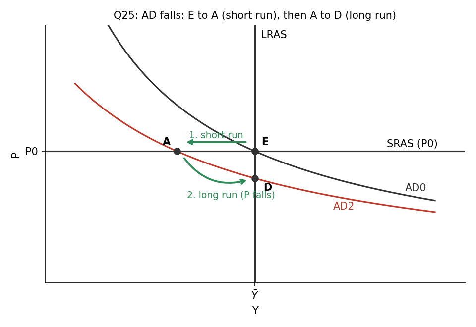
Theory diagram, shapes illustrative. Short run: E to A along SRAS. Long run: A to D along AD2 as prices fall.
- A. True.
- B. False. Reversed order, and D is the long-run point, not the short-run one.
- C. False. A is right for the short run, but B is where meets LRAS (above E), the long-run point after a rise in AD. For a fall in AD the long-run point is D.
- D. False. Returning to E would need AD to come back to . Without policy action the economy ends at D (the lower price level), not E.
🗣️ In plain EnglishA fall in demand first cuts output because prices are slow to move. In time prices fall, output recovers, and the economy ends up with lower prices but the same output as before.
Answer summary
| Q | Topic | Answer |
|---|---|---|
| 1 | MPK < δ: lower saving raises c | A (AI) |
| 2 | AK model: s sets growth | A (AI) |
| 3 | MPK−δ=6% > n+g=4%: raise saving | A (AI) |
| 4 | AB/OA = depreciation rate | A (AI) |
| 5 | Quantity theory long run | A (AI) |
| 6 | Interest rate clears goods market | A (AI) |
| 7 | S > I: interest rate falls | A (AI) |
| 8 | Higher G: interest rate rises | A (AI) |
| 9 | i = 5%, P = 1 | A (AI) |
| 10 | Fisher effect one for one | A (AI) |
| 11 | Higher Y: higher M/P, lower P | A (AI) |
| 12 | Money up: output SR, prices LR | A (AI) |
| 13 | Keynesian cross: G = 260 | A (AI) |
| 14 | LM slope | A (AI) |
| 15 | G multiplier > tax multiplier | A (AI) |
| 16 | Fixed rate: Y unchanged | A (AI) |
| 17 | Phillips: short run only | A (AI) |
| 18 | Hysteresis raises natural rate | A (AI) |
| 19 | SRAS: Y < natural, P < P^e | A (AI) |
| 20 | P falls: ε falls, NX rises | A (AI) |
| 21 | G cut, floating: point D | A (AI) |
| 22 | IS* slopes down | A (AI) |
| 23 | Monetary potency: large d, small f | A (AI) |
| 24 | Vertical LM: ΔY = 0 | A (AI) |
| 25 | AD falls: A then D | A (AI) |
Related Notes
Macro-Economics II · Lec_03-Classical Theory & National Income · Lec_05-Inflation · Lec_06-AS-AD Model & Economic Fluctuations · Lec_07-Aggregate Demand I & the IS-LM Model · Lec_08-Aggregate Demand II & Applying the IS-LM Model · Lec_09-The Open Economy Revisited & Mundell-Fleming Model · Lec_14-Aggregate Supply & the Phillips Curve