
Sample Exam June 2021 — Worked Solutions
- #macro-economics-ii
- #past-paper
- #worked-solution
- #multiple-choice
- #solow-growth
- #is-lm
- #mundell-fleming
- #phillips-curve
- #hysteresis
Sample Exam June 2021 — Worked Solutions
Part of: Macro-Economics II Sample Exam, June 2021 — Macroeconomics II 3058, Dr. Alon Cohen, Tiomkin School of Economics. 25 multiple-choice questions, 4% each, open books. Builds on: Lec_03-Classical Theory & National Income, Lec_06-AS-AD Model & Economic Fluctuations, Lec_07-Aggregate Demand I & the IS-LM Model, Lec_08-Aggregate Demand II & Applying the IS-LM Model, Lec_09-The Open Economy Revisited & Mundell-Fleming Model, Lec_14-Aggregate Supply & the Phillips Curve
Answer key sourceEvery answer below is taken from the official key (all 25 questions are answered there), so no question is AI-solved. The "why each wrong option is wrong" explanations and every callout marked Intuition are my own expansions. Where the official working is terse I have filled in steps but never changed an answer. I checked the arithmetic of Q2, Q3, Q7, Q14, Q24 and Q25 independently and it agrees with the key.
Solow questions have no lecture deckQ1 to Q7 are Solow growth (textbook Ch 8-9). There is no Lec note for it in this vault, so those questions link only to Lec_03-Classical Theory & National Income for the production function background. The wiki-links for Solow concepts do not exist yet.
What this paper tests
| Block | Questions | Core idea |
|---|---|---|
| Solow growth | Q1 to Q7 | Steady state is where . Saving changes levels, only technology changes long-run growth of |
| Sticky prices, AD-AS | Q8 to Q10 | Short run: AS is flat or upward-sloping because of Price Stickiness. Long run: prices adjust and output returns to normal |
| IS-LM | Q11 to Q16 | Slopes, shifts, Crowding Out, and how a price change shifts LM and so gives AD its slope |
| Mundell-Fleming | Q17 to Q20 | Small open economy: floating rate kills fiscal policy, fixed rate kills monetary policy |
| AS and Phillips curve | Q21 to Q25 | Partial stickiness, supply shocks, Sacrifice Ratio, Hysteresis |
Intuition: the one move that unlocks each blockBefore reading options, draw the picture: the Solow diagram (Q1 to Q7), IS-LM (Q11 to Q16), IS*-LM* (Q17 to Q20) or AD-AS (Q8 to Q10, Q21 to Q23). Nearly every wrong option here is the right answer to a different regime, for example the floating-rate result offered in a fixed-rate question.
Q1 — Population growth in Solow
Assume the Solow growth model with no technological progress. The higher the population growth rate is: the _____ the steady-state level of capital per worker, the _____ the growth rate of total income and the growth rate of income per capita is _____
- A. Lower, lower, zero
- B. Higher, higher, higher
- C. Lower, higher, zero
- D. Lower, higher, higher
Answer: C. Lower, higher, zero
Higher raises break-even investment , so the break-even line rotates up and the steady state falls. At the steady state and so are constant (income per capita growth is zero). Total output therefore grows at the rate of , which is , now higher.
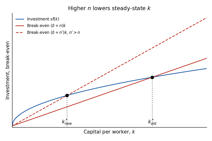
The dashed line is break-even investment after rises. The intersection with moves left.
Why the others are wrong
- A: total income growth equals , which rose, so "lower" is wrong.
- B and D: income per capita growth is zero in a no-technology steady state, not higher.
🗣️ In plain EnglishMore babies means more people to equip with machines, so each worker ends up with less capital than before. But there are more workers, so the whole economy still grows faster. Income per person just sits still.
Q2 — Steady-state income per worker
, saving 10%, depreciation 20%. What is steady-state income per worker?
- A.
- B.
- C.
- D.
Answer: A.
Per worker the production function is . With no population growth or technology the steady state is :
Why the others are wrong
- B is , an intermediate step, not .
- C is itself (), capital per worker rather than income per worker.
- D is the reciprocal of A. It comes from flipping the ratio to .
🗣️ In plain EnglishSet saving equal to wear-and-tear: . Solve for capital, then take the cube root once more to get output per worker. B and C are just stops along the way.
Q3 — Golden-rule saving rate
, saving 25%, depreciation 20%. Should policymakers change the saving rate to reach the golden-rule consumption level?
- A. No
- B. Yes, it should lower it to 20%
- C. Yes, it should increase it to 30%
- D. Yes, it should increase it to 50%
Answer: D. Yes, increase it to 50%
Golden rule: consumption per worker is maximised where . With :
The saving rate that sustains it satisfies :
At the current the economy sits at , well below , so it under-saves.
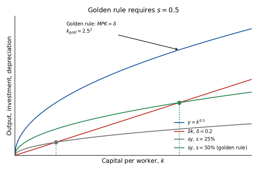
The green line is at , crossing exactly at the golden-rule capital stock.
IntuitionWith Cobb-Douglas the golden-rule saving rate equals the capital share, here . This is a quick check on any such question.
Why the others are wrong
- A: current is not the golden-rule rate.
- B (20%): confuses with . Lowering saving would move the economy further from the golden rule.
- C (30%): points the right way but undershoots, since is required.
🗣️ In plain EnglishThe consumption-maximising capital stock is where an extra machine just replaces its own wear and tear. For this economy that needs a 50% saving rate, and it only saves 25%, so it should save more.
Q4 — Growth of total output
In a Solow model with technological change, population grows at 2% and the efficiency of labor grows at 3%. In the steady state total output grows at ___ percent.
- A. 0
- B. 2
- C. 3
- D. 5
Answer: D. 5
Output per effective worker is constant in the steady state, so grows at the same rate as , which is .
Why the others are wrong
- A (0): the growth rate of output per effective worker, not total output.
- B (2): population growth alone, forgetting technology.
- C (3): the growth rate of output per worker , forgetting population.
🗣️ In plain EnglishTotal output grows with more workers (2%) plus better workers (3%). Add them: 5%. Output per person alone would only grow at 3%.
Q5 — Lower government deficit
Based on Solow with population growth and labor-augmenting technological progress, how would a reduction in the budget deficit affect the steady-state level and growth rate of output per person?
- A. Not alter the level, not alter the growth rate
- B. Increase the level, not alter the growth rate
- C. Increase the level, increase the growth rate
- D. Not alter the level, increase the growth rate
Answer: B. Increase the level, but not the growth rate
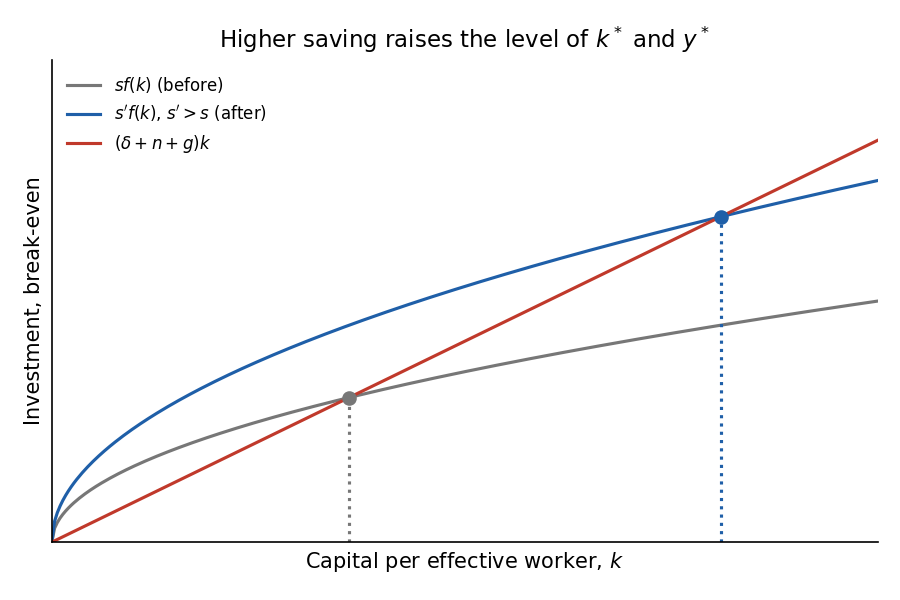
A smaller deficit raises national saving, so rises. The steady-state and hence the level of rise. The long-run growth rate of output per person is set only by technological progress , so it is unchanged. During the transition growth is temporarily faster.
Why the others are wrong
- A: saving does raise the steady-state level.
- C and D: claim saving changes the steady-state growth rate, which Solow denies. Only does that.
🗣️ In plain EnglishSaving more makes the economy richer for good, but not faster-growing for good. It gets a one-off boost to the level and then returns to growing at the technology rate.
Q6 — Can investment sustain growth in living standards?
- A. Yes, when investment exceeds depreciation, capital accumulates and causes sustainable growth
- B. Yes, in the steady state total output increases at the same rate as capital
- C. No, since returns to capital diminish, at some point capital per worker stops growing and so does income per person
- D. No, since under the Solow model investment can never increase the income per person
Answer: C
Diminishing returns mean the investment curve flattens while break-even investment is linear, so the two must cross. Beyond that point, extra capital per worker cannot be sustained and stops rising.
Why the others are wrong
- A: investment above depreciation raises capital only temporarily, until the gap closes. It is not sustainable.
- B: it is true that and both grow at , but that is growth of the total, driven by population and technology, not growth in living standards.
- D: too strong. Investment does raise the level of income per person (see Q5), just not its long-run growth.
🗣️ In plain EnglishEach extra machine adds less than the one before, while replacing machines costs the same each time. So piling on capital runs out of steam, and living standards stop climbing unless technology improves.
Q7 — Growth of wage and rental rate
Depreciation 10%, saving 20%, population growth 2%, technological progress 5%. What are the growth rates of the wage and the rental rate?
- A. 5% and 0%
- B. 5% and 5%
- C. 8% and 20%
- D. 7% and 5%
Answer: A. 5% and 0%
The rental rate equals , and is constant in the steady state, so it does not grow (0%). Factor shares are constant (Euler), so labor's share is fixed. grows at 2% and at , so , the real wage, must grow at .
Why the others are wrong
- B: the rental rate cannot grow at 5%. is constant, so is constant.
- C: 8% and 20% have no basis in the steady-state arithmetic (they just mix parameters).
- D: 7% is the growth of total output, not the wage.
🗣️ In plain EnglishWages rise with productivity per worker (5%), but the return on a machine stays flat (0%) because capital per worker is stuck in the steady state.
Q8 — Why money is not neutral in the short run
Classical theory says output is supply-determined and monetary expansion cannot affect real variables. In the short run both predictions are violated. The main reason:
- A. flexible prices
- B. the use of a different model in the short run
- C. sticky prices
- D. different monetary policy in the short run
Answer: C. Sticky prices
With rigid prices the short-run AS curve is not vertical. Higher demand pushes prices above what was expected, making production more profitable, so firms produce above normal. Equivalently, only some firms can raise prices, so the price rise does not fully absorb the demand rise. See Price Stickiness and Money Neutrality.
Why the others are wrong
- A: flexible prices are the classical assumption that delivers neutrality.
- B: the model differs because of stickiness, but stickiness is the underlying reason.
- D: the policy is not different, the economy's response is.
🗣️ In plain EnglishIf prices could change instantly, extra money would just raise prices. Because many prices are stuck, extra spending makes firms produce more for a while instead.
Q9 — Pessimism shock in AD-AS
All prices are stuck in the short run, economy starts in long-run equilibrium. Pessimism lowers investment and consumption. Short-run and long-run outcomes?
- A. SR: prices unchanged, recession; LR: prices fall, output and unemployment back to normal
- B. SR: prices fall and recession; LR: prices unchanged, output back to normal
- C. SR: prices and output unchanged; LR: prices rise, output above normal
- D. SR: prices unchanged, recession; LR: prices fall but output remains below normal
Answer: A
Lower and shift AD left. Prices are stuck, so output falls (recession). Low output and high unemployment then push prices down over time, SRAS shifts down, and output returns to its natural level at a lower price level.
Why the others are wrong
- B: "all prices stuck" means prices cannot fall in the short run.
- C: the shock is negative, so output cannot stay put, and prices rise only after a positive shock.
- D: if prices fall, output does recover. Output staying below normal in the long run would mean prices never fully adjust.
🗣️ In plain EnglishDemand drops, firms can't cut prices yet so they cut output and jobs. Eventually prices fall and things go back to normal.
Q10 — Adverse supply shock
- A. Regulatory reform lowers the burden on firms
- B. The Central Bank lowers the quantity of money
- C. Labor unions successfully negotiate higher wages for their members
- D. World oil cartel agreement is breached by excessive production by its members
Answer: C
An adverse supply shock raises firms' costs, shifting SRAS up. Higher wages are a rise in the price of labor services, so they do exactly that.
Why the others are wrong
- A: lower costs: a favorable supply shock.
- B: monetary policy shifts AD, not AS.
- D: over-production lowers oil prices, a favorable supply shock.
🗣️ In plain EnglishA supply shock is anything that makes it more expensive to produce. Higher wages do that. Cheaper oil and less red tape do the opposite.
Q11 — How the long-run equilibrium is restored in IS-LM
Pandemic lowers consumption and investment. How is long-run equilibrium normally restored?
- A. The government applies expansionary fiscal policy, shifting the IS curve leftward
- B. The central bank takes expansionary monetary measures, shifting the LM curve leftward
- C. Prices fall, shifting the IS curve rightward
- D. Prices fall, shifting the LM curve rightward
Answer: D. Prices fall, shifting LM rightward
The fall in and shifts IS left, lowering and . Output below normal pushes prices down in the long run, so real money balances rise. That acts like a monetary expansion and shifts LM right, lowering further and boosting investment until is back to normal.
Why the others are wrong
- A: expansionary fiscal policy shifts IS rightward, and it is a policy choice, not the "normal" automatic adjustment.
- B: expansionary monetary policy shifts LM rightward, not leftward.
- C: price changes move the LM curve (through ), not IS.
🗣️ In plain EnglishWhen prices fall, the same money buys more, which acts like the central bank adding money. Interest rates drop and investment picks back up.
Q12 — Why LM slopes upward
- A. When rises, falls so falls
- B. When rises, demand for money rises so rises
- C. When increases falls, so increases and rises
- D. When falls falls, so falls as well
Answer: B
Real money supply is fixed. Higher income raises money demand, taking the money market out of equilibrium. Only a higher interest rate, which raises the opportunity cost of holding money and so lowers quantity demanded, restores it. See LM Curve and Liquidity Preference.
Why the others are wrong
- A: this explains the negative slope of the IS curve.
- C: describes a shift of LM from a monetary expansion, not its slope.
- D: money supply does not move with income here. The mechanism is on the money demand side.
🗣️ In plain EnglishRicher people want more cash for transactions. With the money supply fixed, the only way to make people hold less is a higher interest rate.
Q13 — Stronger preference for cash
- A. Interest rate rises, output falls
- B. Interest rate falls, output rises
- C. Interest rate rises, output rises
- D. Interest rate falls, output falls
Answer: A
Stronger liquidity preference raises money demand at each , which is a monetary contraction: LM shifts up and left. The interest rate rises, investment falls, output falls.
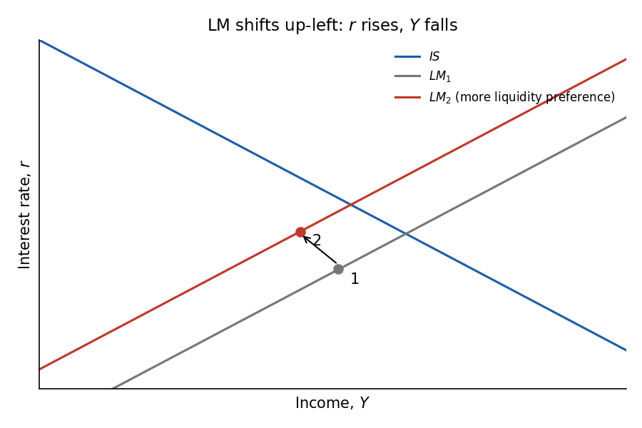
Why the others are wrong
- B: the direction of a monetary expansion.
- C: IS is unchanged, so moving up the IS curve must lower when rises.
- D: cannot fall when money demand rises with a fixed supply.
🗣️ In plain EnglishEveryone hoarding cash is like the central bank removing money. Borrowing gets pricier and output falls.
Q14 — Multiplier of 4, but Y rises only by 300
The Keynesian multiplier is 4. Government raises by $100B. Output rises by $300B. What happened to investment?
- A. Crowded out by 100
- B. Crowded out by 25
- C. Has not changed
- D. Increased by 100
Answer: B. Crowded out by 25
A multiplier of 4 means . Then:
Why the others are wrong
- A (100): the naive error: the fixed- increase is , and is not the investment fall, because the fall in also reduces consumption through the multiplier. The 100 is the output loss, the investment loss is .
- C: if investment had not changed, would rise by the full 400.
- D: investment rising would make rise by more than 400.
🗣️ In plain EnglishGovernment spending would have lifted output by 400, but it only rose 300, so something dragged it back. Account for the knock-on effect on consumption and the culprit is investment falling by 25.
Q15 — Central bank response to fiscal contraction
Government cuts spending. The central bank wants to mitigate changes in the interest rate.
- A. Do nothing
- B. Apply expansionary monetary policy
- C. Apply contractionary monetary policy
- D. Shift the LM curve rightward
Answer: C
Contractionary fiscal policy shifts IS left and lowers and . To keep from falling, the central bank must push up, which means contracting the money supply and shifting LM left. (Output would fall even more, so it stabilises at the cost of .)
Why the others are wrong
- A: would fall.
- B and D: expansion shifts LM right and lowers even more.
🗣️ In plain EnglishSpending cuts push interest rates down. To hold rates steady the central bank must do the opposite and tighten money.
Q16 — Why AD slopes downward
- A. the interest rate effect, which rises with , driving investment downward
- B. the interest rate effect, which moves inversely to and investments
- C. the quantity theory of money, whereby higher lowers purchasing power
- D. the exchange rate effect, which rises with , driving net export downward
Answer: A
A higher lowers and shifts LM left. The interest rate rises, investment falls, and so does output. That gives AD its negative slope. See Aggregate Demand Curve.
Why the others are wrong
- B: the interest rate moves with (not inversely).
- C: the quantity theory is a long-run relationship, not the IS-LM mechanism asked about.
- D: an exchange-rate effect belongs to the open-economy extension, not to the closed-economy IS-LM insight asked about.
🗣️ In plain EnglishHigher prices make the money supply worth less, so interest rates climb, investment drops, and total demand falls.
Q17 — Exchange rate appreciation in a small open economy
Appreciation of is expected to ___ net exports and induce a movement ___ the ___ curve.
- A. increase, along, IS*
- B. increase, of, IS*
- C. decrease, along, IS*
- D. decrease, along, LM*
Answer: C. Decrease, along, IS*
Domestic goods are priced in domestic currency, so appreciation makes them more expensive abroad and foreign goods cheaper at home: falls. A change in is a movement along IS* because is on the vertical axis. See IS* Curve and Net Exports.
Why the others are wrong
- A and B: appreciation lowers, not raises, net exports. B also gets "of" wrong.
- D: LM* is vertical in space and does not depend on .
🗣️ In plain EnglishA stronger currency makes our goods pricey and imports cheap, so net exports fall. It slides us along the IS* curve.
Q18 — Tax rise under a fixed exchange rate
Mundell-Fleming with a fixed exchange rate. Benchmark equilibrium is point C. The government raises taxes. What happens?
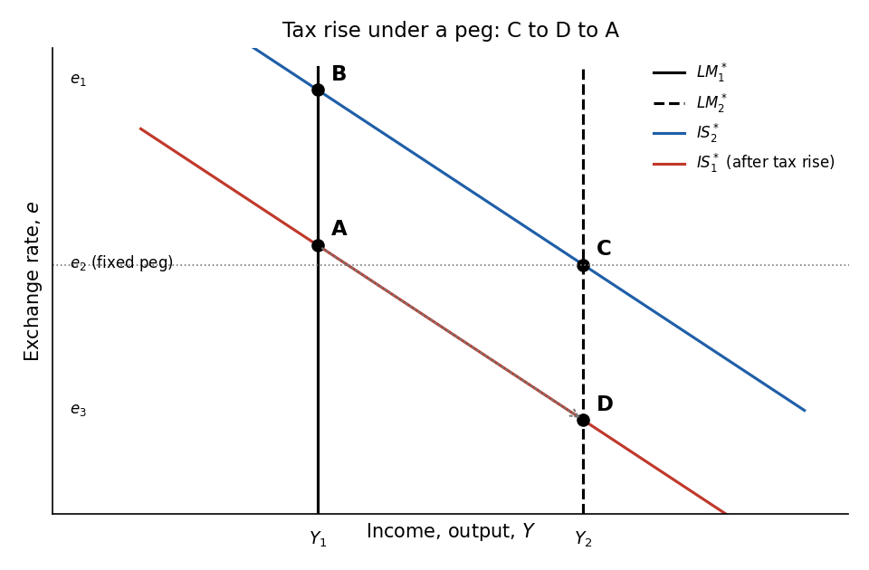
Redrawn from the exam figure. C is on and at . After the tax rise shifts left to .
- A. The central bank will apply contractionary monetary policy, leading to point B
- B. The central bank will not intervene, leading to point D
- C. The central bank will buy foreign currency and sell local currency, leading to point A
- D. The central bank will buy local currency and sell foreign currency, leading to point A
Answer: D
Higher taxes shift IS* left, which puts downward pressure on the local currency (point D at ). To defend the peg at the central bank must support the currency: it buys local currency and sells foreign currency, which shrinks the money supply and moves LM* left. The new equilibrium is A, with the original restored but lower . See Fixed Exchange Rate.
Why the others are wrong
- A (point B): B lies on , which ignores the fiscal shift. The tax rise has already moved IS* to .
- B (point D): no intervention is the floating regime outcome, with falling to . Under a peg the bank must act.
- C: buying foreign currency and selling local would expand the money supply, pushing the currency down further.
🗣️ In plain EnglishUnder a peg the central bank can't let the currency slide, so it soaks up its own currency, which shrinks the money supply. Fiscal policy ends up changing output, and the exchange rate stays where it was.
Q19 — Helping import-competing industries (floating rate)
- A. Cancel import quotas
- B. Set import quotas, however this will cause unemployment in export industries because of the appreciation of the exchange rate
- C. Set import quotas, however this will cause unemployment in export industries because of the depreciation of the exchange rate
- D. Set import quotas and increase thereby total output
Answer: B
A quota cuts imports and shifts IS* right. Under floating rates the currency appreciates, which lowers exports until net exports are back where they started. Both imports and exports are now lower: import-competing firms gain, export firms lose. is unchanged, so unemployment overall is unchanged, only its composition shifts.
Why the others are wrong
- A: removing quotas hurts the very industries the government wants to help.
- C: the currency appreciates (IS* shifts right), it does not depreciate.
- D: under floating rates trade policy cannot raise total output.
🗣️ In plain EnglishQuotas protect some jobs but cost others: the stronger currency makes exports uncompetitive. In total nothing improves, the unemployed just move to different industries.
Q20 — Tax cut, small open economy, floating rate
Perfect capital mobility, flexible exchange rate, starting at natural output with balanced trade. Impact of a tax cut on output and the trade balance in the short and long run?
- A. Output stays the same and there is trade deficit, both in the short and long run
- B. Output increases in SR and returns to normal in LR; deficit in SR and balance restored in LR
- C. Output stays the same in both; deficit created in SR and balance restored in LR
- D. Output increases in SR and returns to normal in LR; deficit in both SR and LR
Answer: A
Under floating rates and perfect capital mobility fiscal policy cannot change output. The tax cut shifts IS* right, the currency appreciates, and net exports fall by exactly as much as the stimulus. is unchanged, with a trade deficit (higher consumption and imports, lower exports). The long run is no different from the short run.
Why the others are wrong
- B and D: claim output rises in the short run, but with floating rates the appreciation crowds out net exports one for one.
- C: claims the deficit disappears in the long run. Nothing in the model restores trade balance, as is already at its natural level, so the exchange rate stays appreciated.
🗣️ In plain EnglishA tax cut makes the currency stronger, which wipes out the boost to output by hurting exports. Output doesn't move, but the country now runs a trade deficit for good.
Q21 — Partial stickiness and returning to long-run equilibrium
Sticky prices for only some of the firms. Expansionary policy in the short run ___ inflationary, and the driving force behind the return to long-run equilibrium is a change in ___
- A. is not, prices
- B. is, prices' expectations
- C. is, prices
- D. is not, prices' expectations
Answer: B. Is, prices' expectations
With only some firms sticky, SRAS slopes upward, so higher comes with higher : any expansion is inflationary (though less so when output is below normal). Returning to the long run requires expectations to adjust: higher prices make people revise expected prices up, which shifts SRAS up. See Sticky-Price Model and SRAS Curve.
Why the others are wrong
- A and D: an upward-sloping SRAS means expansion does raise prices.
- C: actual prices already moved in the short run. What returns the economy to normal is the adjustment of expectations, which shifts the curve itself.
🗣️ In plain EnglishSome prices do rise, so expansion is inflationary. The economy only settles when everyone updates what they expect prices to be.
Q22 — Fraction of sticky firms falls
What is the plausible prediction about the magnitude and duration of the business cycle as falls?
- A. Greater magnitude, longer duration
- B. Greater magnitude, shorter duration
- C. Lower magnitude, longer duration
- D. Lower magnitude, shorter duration
Answer: D. Lower magnitude, shorter duration
A small means almost all firms are flexible, so SRAS becomes nearly vertical. A demand shock then mostly changes prices and barely changes output, so the deviation is small and the return to normal is quick.
Why the others are wrong
- A, B, C: each pairs at least one of the two features backwards. Fewer sticky firms means less output deviation and faster convergence on both counts.
🗣️ In plain EnglishThe fewer firms with stuck prices, the more a demand shock gets absorbed by prices instead of output. Recessions are milder and shorter.
Q23 — Cost-push inflation
Starting from long-run equilibrium at A with output and price level , a cost-push inflation would be a shift from:
- A. AD1 to AD2
- B. AD1 to AD3
- C. AS1 to AS2
- D. AS1 to AS3
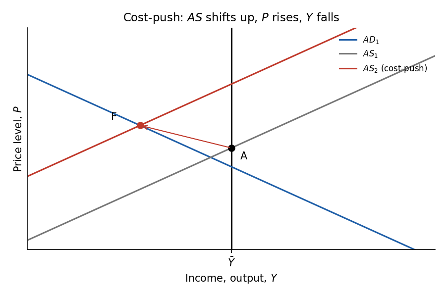
Schematic only (the exam figure has more curves). AS1 to AS2 is an upward shift of AS, raising and lowering at first.
Answer: C. AS1 to AS2
Cost-push inflation comes from a supply shock that raises costs, shifting AS up (AS2 passes through , above ). See Cost-Push Inflation and Supply Shock.
Why the others are wrong
- A: AD1 to AD2 is a rise in demand: Demand-Pull Inflation.
- B: AD1 to AD3 is a fall in demand, lowering prices.
- D: AS1 to AS3 is a favorable supply shock (lower costs), lowering .
🗣️ In plain EnglishIf costs jump (wages, oil) prices rise even though demand hasn't changed. That is an upward shift in supply, the opposite of demand-pull.
Q24 — Sacrifice ratio
Phillips curve . Okun's law: each percentage point of extra unemployment costs 2% of GDP. What is the sacrifice ratio?
- A. 6
- B. 0
- C. 4
- D. 2
Answer: C. 4
Cutting inflation by 1 point requires in percentage-point terms, that is unemployment 2 points above its natural rate. Okun's law: of GDP lost per point of disinflation. See Sacrifice Ratio and Okun's Law.
Why the others are wrong
- D (2): stops after the first step: it reads the unemployment cost (2 points) or the Okun coefficient as the answer.
- A (6) and B (0): do not follow from combining the two coefficients (, then ).
🗣️ In plain EnglishTo drop inflation by 1 point you need 2 extra points of unemployment, and each extra point costs 2% of GDP. Multiply: 4% of GDP.
Q25 — Hysteresis
Normal unemployment is the moving average of the previous two years. . The Fed lowers inflation by 1% in period 1 and keeps it there. By how much does the normal unemployment rate in period 4 exceed its original level?
- A. 1.25%
- B. 1.5%
- C. 1%
- D. 1.375%
| Period | 0 | 1 | 2 | 3 | 4 |
|---|---|---|---|---|---|
| Actual u-rate | |||||
| Normal u-rate |
Answer: A. 1.25%
A 1-point cut in inflation costs 2 extra points of unemployment, so actual in period 1 is . From period 2 the Fed wants inflation held constant, so exactly. The normal rate each year is the average of the previous two actual rates:
- period 2:
- period 3:
- period 4:
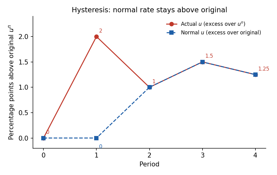
The normal rate overshoots to 1.5 and is on its way to a permanent increase.
Why the others are wrong
- B (1.5%): the period 3 value, one period too early.
- C (1%): the period 2 value, two periods too early.
- D (1.375%): the average of periods 3 and 4, a made-up smoothing that does not follow the rule.
IntuitionHysteresis turns a short-run Phillips trade-off into a lasting one. The official key does not answer the paper's extra "Bonus" prompt (prove convergence to 1.333...), so it is left out here.
🗣️ In plain EnglishFighting inflation causes a recession, and the recession drags the "normal" unemployment rate up with it. Four years on, normal unemployment is still 1.25 points higher than before.
Recap table
| Q | Topic | Answer |
|---|---|---|
| 1 | Higher in Solow | C |
| 2 | Steady-state | A |
| 3 | Golden-rule saving | D |
| 4 | Total output growth | D |
| 5 | Lower deficit | B |
| 6 | Investment and sustained growth | C |
| 7 | Wage and rental growth | A |
| 8 | Why money matters short run | C |
| 9 | Pessimism shock | A |
| 10 | Adverse supply shock | C |
| 11 | Restoring LR in IS-LM | D |
| 12 | LM slope | B |
| 13 | More cash preference | A |
| 14 | Crowding out | B |
| 15 | Offsetting fiscal cut | C |
| 16 | AD slope | A |
| 17 | Appreciation | C |
| 18 | Tax rise, fixed | D |
| 19 | Import quotas | B |
| 20 | Tax cut, floating | A |
| 21 | Partial stickiness | B |
| 22 | Falling | D |
| 23 | Cost-push | C |
| 24 | Sacrifice ratio | C |
| 25 | Hysteresis | A |
Related notes
Macro-Economics II · Lec_03-Classical Theory & National Income · Lec_06-AS-AD Model & Economic Fluctuations · Lec_07-Aggregate Demand I & the IS-LM Model · Lec_08-Aggregate Demand II & Applying the IS-LM Model · Lec_09-The Open Economy Revisited & Mundell-Fleming Model · Lec_14-Aggregate Supply & the Phillips Curve