
Moed A 2022 — Worked Solutions
- #macro-economics-ii
- #past-paper
- #worked-solution
- #multiple-choice
- #ai-solved
- #classical-theory
- #solow-growth
- #is-lm
- #mundell-fleming
- #phillips-curve
Moed A 2022 — Worked Solutions
Part of: Macro-Economics II Moed A, 16 June 2022 (Reichman University, Tiomkin School of Economics) | Macroeconomics II 3058 | Dr. Alon Cohen | 25 multiple-choice questions, 4% each, 2.5 hours, open books, simple calculator Key concepts: Loanable Funds Market, Quantity Theory of Money, Velocity of Money, Fisher Effect, Classical Dichotomy, Keynesian Cross, Inventory Adjustment, Liquidity Preference, IS-LM Equilibrium, AD-AS Model, Mundell-Fleming Model, Fixed Exchange Rate, Floating Exchange Rate, Large Open Economy, Sticky-Price Model, Phillips Curve, Hysteresis Builds on: Lec_03-Classical Theory & National Income, Lec_05-Inflation, Lec_06-AS-AD Model & Economic Fluctuations, Lec_07-Aggregate Demand I & the IS-LM Model, Lec_08-Aggregate Demand II & Applying the IS-LM Model, Lec_09-The Open Economy Revisited & Mundell-Fleming Model, Lec_14-Aggregate Supply & the Phillips Curve
AI-written answers, not official. Check before relying on them.All 25 questions (Q1 to Q25) are AI-solved. There is no official key for this sitting, and the paper is not a tofes 0 paper (its header says nothing about tofes 0, and in the keyed 2022 Moed B paper the official answer is not always the first option). So the "answer printed first" cross-check does not apply, and every answer below stands on its own working, with a confidence level per question. Q5 to Q9 (Solow growth) have no lecture deck in this vault, so those rest on standard Solow results rather than on a lecture note.
Yellow highlights in the source PDFThe question PDF carries yellow highlighting on one option per question. Its author is unknown, so it is not treated as an official key. For transparency: the highlighted options agree with the answers worked out below on all 25 questions. I saw the highlights while reading the pages, so the working below is not fully blind. Each answer is nonetheless derived from the model, not copied from the highlight.
Two wording problems in the paper itself
- Q11: options A and B are word-for-word identical (both correct). Pick either.
- Q15: "be only inflationary" is loose, since the interest rate also rises in the long run. It is still the best of the four.
What this paper tests
| Questions | Topic | Lecture |
|---|---|---|
| Q1, Q3 | Classical loanable funds, saving shocks, Fisher effect | Lec 03, Lec 05 |
| Q2, Q4 | Quantity theory, velocity, expected future money | Lec 05 |
| Q5 to Q9 | Solow growth: golden rule, steady state, factor prices | No lecture deck (Ch 8-9) |
| Q10, Q22, Q23 | AD-AS, velocity shock, sticky prices, policy and inflation | Lec 06, Lec 14 |
| Q11 to Q14 | Keynesian cross, LM curve, money transmission, IS-LM numbers | Lec 07, Lec 08 |
| Q15 | IS-LM to the long run | Lec 08 |
| Q16 to Q21 | Mundell-Fleming: small open, fixed and floating, large open economy | Lec 09 |
| Q24, Q25 | Phillips curve, hysteresis | Lec 14 |
Answer sheet (AI-solved)
| Q | 1 | 2 | 3 | 4 | 5 | 6 | 7 | 8 | 9 | 10 | 11 | 12 | 13 |
|---|---|---|---|---|---|---|---|---|---|---|---|---|---|
| Ans | B | A | B | C | B | A | D | C | C | A | A | C | B |
| Confidence | High | High | High | Med-high | High | High | High | High | Medium | Med-high | High | High | Med-high |
| Q | 14 | 15 | 16 | 17 | 18 | 19 | 20 | 21 | 22 | 23 | 24 | 25 |
|---|---|---|---|---|---|---|---|---|---|---|---|---|
| Ans | C | A | B | C | C | B | B | C | B | A | D | B |
| Confidence | High | Medium | High | High | Med-high | High | Med-high | High | Med-high | Med-high | High | High |
Q1 — The classical loanable funds market
Consider the market of goods and services and the market of loanable funds under the classical theory.
- A. Both markets are cleared by the interest rate: the higher it is, the lower is the overall output level, Y
- B. Both markets are cleared by the interest rate, but overall output Y is not affected by it
- C. Higher government deficit increases interest rate, increases the quantity of loanable funds, national investments, and overall output level Y.
- D. Higher government deficit increases interest rate, lowers the quantity of loanable funds, national investments, and overall output level Y.
AI-written answer, not official. Check before relying on it.
Answer: B (confidence: high)
In the classical model output is fixed by the production function, . The interest rate then adjusts so that saving equals investment, , which is the same as clearing the goods market, because and . So clears both markets, but it has no effect on .
Why the wrong options fail
- A makes output depend on . In the classical model is set on the supply side.
- C has a deficit raising investment and output. A deficit lowers public saving, shifting loanable-funds supply left, so rises and investment falls (crowding out). does not move.
- D gets the rise in and the fall in investment right, but wrongly says falls. is unchanged.
🗣️ In plain EnglishIn the classical world, output is decided by how much capital and labour you have, not by the interest rate. The interest rate just balances saving and investment. A bigger deficit pushes the rate up and crowds out investment, but it leaves total output alone.
Q2 — Quantity theory with accelerating velocity
According to the quantity theory of money, if money is growing at a 10 percent rate and real output is growing at a 3 percent rate, but velocity is growing at increasingly faster rates over time as a result of financial innovation, the rate of inflation must be
- A. increasing.
- B. decreasing.
- C. constant.
- D. 7%.
AI-written answer, not official. Check before relying on it.
Answer: A (confidence: high)
From , in growth rates:
where is velocity growth. With and fixed, . Velocity growth is itself rising over time, so rises over time.
Why the wrong options fail
- B has the sign backwards: extra velocity growth adds to inflation.
- C needs constant.
- D (7%) is the textbook answer only when velocity is constant (). Here it is not, and it is accelerating, so inflation is above 7% and climbing.
🗣️ In plain EnglishIf the same money changes hands faster and faster, prices get pushed up by more and more. So inflation isn't stuck at 7%, it keeps climbing.
Q3 — A tax break on saving: money growth and nominal rates
The government implemented a tax relief on long-term savings, which lowered households' consumption. Under the classical theory, if the Central Bank will
- A. keep the same money growth rate, nominal interest rate could remain unchanged.
- B. lower the money growth rate, nominal interest rate will necessarily fall.
- C. lower the money growth rate, nominal interest rate will necessarily rise.
- D. lower the money growth rate, nominal interest rate could remain unchanged.
AI-written answer, not official. Check before relying on it.
Answer: B (confidence: high)
Use the Fisher equation, .
- Lower consumption means higher private saving, so national saving rises. Loanable-funds supply shifts right and the real rate falls. (Output is fixed, so this is the only real effect.)
- With constant velocity and fixed output, . Cutting money growth lowers .
Both and fall, so must fall.
Why the wrong options fail
- A keeps (so ) unchanged, but still falls, so falls. It cannot "remain unchanged".
- C has rising. Neither component rises.
- D is right that falls but wrong that could stay put: both pieces of move down together, so there is no offsetting force.
🗣️ In plain EnglishThe tax break means more saving, so the real interest rate drops. Slower money growth also drops inflation. The nominal rate is real rate plus inflation, so with both falling it has to fall.
Q4 — Announced versus actual money growth
Under the classical theory, if the Fed presently increases M, or, alternatively, declares it will increase M next year, then both options bear opposite effects over current prices.
- A. True. Increasing M at the present will proportionally increase prices, whereas a mere declaration of future increase of M will decrease current prices.
- B. True. Increasing M at the present will proportionally decrease prices, whereas a mere declaration of future increase of M will increase current prices.
- C. False. In both cases current prices will rise.
- D. False. Increasing M at the present will proportionally increase prices, whereas a mere declaration of future increase of M will not affect current prices.
AI-written answer, not official. Check before relying on it.
Answer: C (confidence: medium-high)
Money market equilibrium is with and fixed.
- Increase now: real money demand is unchanged, so rises in proportion to .
- Announce an increase next year: expected inflation rises today, which raises the nominal rate and lowers money demand today. At the current there is excess supply of money, people spend it, and rises now, before has moved. Lec_05-Inflation makes exactly this point.
So the effects are not opposite: both raise current prices.
Why the wrong options fail
- A and B claim opposite effects. B also has a present increase in lowering prices, which breaks the quantity theory.
- D has the present increase right but says the announcement has no effect. It works through expected inflation and the nominal rate.
🗣️ In plain EnglishPrices don't wait for the printing press. If everyone expects more money next year, they expect more inflation, hold less cash today and spend it, so prices go up now too.
Q5 — The saving rate at the golden rule
Under Solow growth model with no technological innovation, assume that consumption is maximized, and . Income per worker is given by . What is the saving rate ?
- A. 0.1
- B. 0.5
- C. 0.05
- D. 0.25
AI-written answer, not official. Check before relying on it. Outside the lecture notes: Solow growth (Ch 8-9) has no lecture deck, so this uses the standard golden-rule result.
Answer: B, (confidence: high)
Consumption is maximised at the golden rule, where the marginal product of capital equals the break-even rate:
With , :
In steady state saving equals break-even investment, :
ShortcutFor Cobb-Douglas the golden-rule saving rate is , independent of and .
Why the wrong options fail
- A (0.1) and C (0.05) come from mixing up with the saving rate.
- D (0.25) is the golden-rule rate for , as in a different exercise. Here .
🗣️ In plain EnglishTo get the most consumption forever, a Cobb-Douglas economy saves a share equal to capital's exponent, here half its income.
Q6 — Output per worker growth in steady state
In the Solow growth model, an economy in the steady state with a population growth rate of but no technological growth will exhibit a growth rate of output per worker at rate:
- A.
- B.
- C.
- D.
AI-written answer, not official. Check before relying on it. Outside the lecture notes (no Solow deck).
Answer: A (confidence: high)
In the steady state, capital per worker is constant, so output per worker is constant. Total output grows at , but per worker output grows at .
Why the wrong options fail
- B () is the growth of total and , not of .
- C () and D () are the break-even investment rate, not a growth rate of anything per worker.
🗣️ In plain EnglishWithout new technology, the economy settles where capital per worker stops rising, so output per worker is flat. The economy as a whole grows with the population, but each person doesn't get richer.
Q7 — The only source of persistent growth in living standards
According to the Solow model, persistently rising living standards (income per person) can only be explained by:
- A. population growth
- B. population growth and capital accumulation
- C. high saving rates
- D. technological progress
AI-written answer, not official. Check before relying on it. Outside the lecture notes (no Solow deck).
Answer: D (confidence: high)
Diminishing returns to capital mean more saving or capital only raises the level of income per person for a while, until a new steady state is reached. Population growth actually spreads capital thinner. Only technological progress () lets grow forever.
Why the wrong options fail
- A and B include population growth, which lowers steady-state income per worker.
- C a higher saving rate gives a one-time rise in the level, then growth returns to its old rate.
🗣️ In plain EnglishSaving more or adding people only gets you to a higher plateau. To keep climbing forever you need better technology.
Q8 — Factor price growth rates
Solow's growth theory suggests that real wage grows at the rate of ___, and the real rental price grows at the rate of ___.
- A. technological innovation ; technological innovation
- B. technological innovation , population growth
- C. technological innovation , 0
- D. 0, population growth
AI-written answer, not official. Check before relying on it. Outside the lecture notes (no Solow deck).
Answer: C (confidence: high)
With and labour efficiency growing at :
- Real wage . In steady state grows at , so grows at .
- Real rental price . In steady state and both grow at , so is constant and grows at 0.
Why the wrong options fail
- A gives capital's price growth . is constant, so is flat.
- B and D bring in , but affects only the level of factor prices (through ), not their growth rates.
🗣️ In plain EnglishWorkers get more productive over time, so wages rise at the pace of technology. Capital doesn't get more productive per unit, so its rental price stays put.
Q9 — Does capital accumulation give permanent growth?
Capital accumulation underlies Solow's permanent growth of the standard of living.
- A. True. Investment in capital increases the national income and income per person
- B. True, but only if population grows as well, so that investment increases capital to equip new workers
- C. False. Investment in capital can underlie permanent growth only if investment exhibits constant returns to scale, which is not the case in Solow model
- D. False. Investment in capital can underlie permanent growth only if saving rate can be affected, which is not the case in Solow model
AI-written answer, not official. Check before relying on it. Outside the lecture notes (no Solow deck). Confidence is medium because option C is loosely worded.
Answer: C (confidence: medium)
The statement is false. Capital has diminishing returns: each extra unit of capital per worker adds less output, so eventually only just covers break-even investment and stops growing. Permanent growth would need capital's returns not to diminish (as in an AK model), which is not the Solow set-up. Option C says this, though "constant returns to scale" is sloppy: the Solow production function is constant returns in and together. The intended meaning is constant returns to capital alone.
Why the wrong options fail
- A confuses a higher level with permanent growth.
- B population growth makes things worse per worker, not better.
- D the saving rate can be changed (policy, taxes), and changing it shifts only the level, not the long-run growth rate. So the stated reason is wrong.
🗣️ In plain EnglishPiling up machines helps at first, but each extra machine helps less than the last. Eventually growth runs out of steam, so capital alone can't deliver growth forever.
Q10 — A fall in velocity and two central banks
Consider the AD-AS model with overall fixed prices in the short run. If Central Bank A cares only about keeping the price level stable and Central Bank B cares only about keeping output at its natural level, then in response to an exogenous decrease in the velocity of money:
- A. both Central Bank A and Central Bank B should increase the quantity of money.
- B. Central Bank A should increase the quantity of money whereas Central Bank B should keep it stable.
- C. Central Bank A should keep the quantity of money stable whereas Central Bank B should increase it.
- D. both Central Bank A and Central Bank B should keep the quantity of money stable.
AI-written answer, not official. Check before relying on it.
Answer: A (confidence: medium-high)
From , a fall in shifts AD left. With sticky prices, output falls below . Leaving alone lets prices fall over time to restore (self-correction, per Lec_06-AS-AD Model & Economic Fluctuations).
- Bank B (output): raise to shift AD back to its old position, so immediately.
- Bank A (price level): if is left alone, the price level must fall to restore . To keep it from moving, AD must be put back, which also needs a rise in offsetting the drop in .
Offsetting the fall in with higher keeps constant, so both goals are served by the same action.
Why the wrong options fail
- B says Bank B does nothing, but then output stays below until prices fall.
- C says Bank A does nothing, but then the price level has to fall.
- D leaves the demand shock to play out, hurting both goals.
🗣️ In plain EnglishIf people spend each dollar more slowly, total spending drops. Printing more money makes up the difference, which keeps both output and the price level where they were.
Q11 — Keynesian cross at Y₃
Consider the following Keynesian Cross (planned expenditure PE against income Y, with the 45-degree actual-expenditure line; the lines cross at , and ). Suppose that the output level is . The market for goods and services will converge to equilibrium due to
- A. unexpected increase of inventory, which will induce firm to slow down production rate
- B. unexpected increase of inventory, which will induce firm to slow down production rate
- C. a fall in the price level, which will increase planned expenditure
- D. a rise in the price level, which will decrease planned expenditure
The graph (read from the PDF): the 45-degree actual-expenditure line and a flatter planned-expenditure line starting at on the vertical axis. They cross at . At , actual expenditure is and planned expenditure is .
AI-written answer, not official. Check before relying on it.
Answer: A (B is identical and equally correct; confidence: high)
At , actual expenditure (= output) exceeds planned expenditure . The gap is unplanned inventory investment: goods produced but not sold. Firms respond by cutting production, so falls towards , where actual equals planned. See Lec_07-Aggregate Demand I & the IS-LM Model.
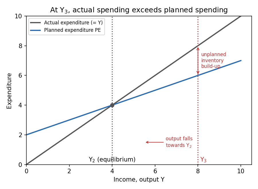
At firms are producing more than is being bought. The unsold stock piles up and output is cut until .
Why the wrong options fail
- B is a duplicate of A (a typo in the paper). It is correct too.
- C and D bring in the price level. The Keynesian cross holds prices fixed, so convergence works through inventories and output, not prices.
🗣️ In plain EnglishIf firms make more than people plan to buy, unsold stock builds up. They respond by producing less, and output slides down to the point where output equals planned spending.
Q12 — Why a higher income raises the interest rate (LM)
The LM curve suggests that if income rises interest rate must rise, due to
- A. a decrease in M
- B. an increase of P
- C. the sale of bonds triggered by excess demand for money
- D. the purchase of bonds triggered by excess supply of money
AI-written answer, not official. Check before relying on it.
Answer: C (confidence: high)
Along the LM curve and are fixed. Higher income raises money demand , so there is excess demand for money. People sell bonds to get cash, bond prices fall, and the interest rate rises until money demand equals the fixed supply again.
Why the wrong options fail
- A and B change the real money supply, which shifts LM. The question asks about movement along LM.
- D has the process in reverse: an excess supply of money would push down.
🗣️ In plain EnglishRicher people want to hold more cash. To get it they sell bonds, which pushes the interest rate up.
Q13 — How monetary expansion raises output in a closed economy
In a closed economy in the short run, the Central Bank's ability to boost output level Y by expanding M is enabled primarily by
- A. the fact that when real balances increase, price level falls and so the demand for goods and services rises
- B. the effect of the interest rate on investments
- C. an increase in the planned expenditure, which lowers the inventory and induces firms to produce more
- D. a rightward shift of the IS and AD curves
AI-written answer, not official. Check before relying on it.
Answer: B (confidence: medium-high)
The transmission mechanism is: higher means higher real balances (with fixed in the short run), the LM curve shifts right, the interest rate falls, investment rises, and so does (via the multiplier). The interest-rate-to-investment link is the channel that makes money matter for output. See Lec_08-Aggregate Demand II & Applying the IS-LM Model.
Why the wrong options fail
- A is the price-level route behind the AD curve's slope. In the short run here prices are fixed.
- C describes the Keynesian-cross adjustment after spending rises. It is a consequence, not the source: the source is the fall in .
- D money does not shift IS. It shifts LM (and AD). IS only moves with , or autonomous spending.
🗣️ In plain EnglishMore money pushes interest rates down. Cheaper borrowing makes firms invest more, and that lifts output.
Q14 — An IS-LM calculation
If the IS curve is given by , the money demand function is given by , the money supply is 1,000, and the price level is 2, then if the money supply is raised to 1,200, equilibrium income rises by:
- A. 200 and the interest rate falls by 2 percent
- B. 100 and the interest rate falls by 1 percent
- C. 50 and the interest rate falls by 0.5 percent
- D. 200 and the interest rate remains unchanged
AI-written answer, not official. Check before relying on it.
Answer: C (confidence: high)
LM: . IS: , i.e. .
Before (): adding and gives , so
After (): , so
Income rises by 50 and the interest rate falls by 0.5 percentage point (6% to 5.5%).
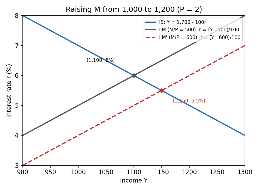
LM shifts right by 100 at each ; equilibrium moves down the IS curve from (1,100; 6%) to (1,150; 5.5%).
Why the wrong options fail
- A and D treat the 200 rise in as a 200 rise in . It is that matters (a 100 rise), and the IS curve absorbs half of the shift.
- B is the 100 horizontal shift of the LM curve itself, not the new equilibrium: the downward-sloping IS curve means rises by only half of that.
- D also wrongly keeps constant, but with a downward-sloping IS curve, must fall for to rise.
🗣️ In plain EnglishMore money in real terms pushes the LM curve out by 100, but because IS slopes down it only lets income rise by 50, with the interest rate dipping by half a point.
Q15 — Fiscal expansion from point B, long run
Consider a closed economy with a vertical LRAS at and IS-LM curves. Suppose that the economy is at equilibrium point B. Fiscal expansion, in the long run, will
- A. be only inflationary
- B. increase both output and interest rate
- C. increase output, interest rate and prices
- D. not change anything in the economy
The graph (read from the PDF): (left of LRAS), (on LRAS), (on LRAS, higher ), (right of LRAS).
AI-written answer, not official. Check before relying on it.
Answer: A (confidence: medium, because of the loose wording)
Fiscal expansion shifts IS from to .
- Short run: economy moves from B to D. Income rises above and rises.
- Long run: pushes the price level up. Real balances fall, so LM shifts left from to , to point C.
At C output is back at , so there is no real output effect. The price level is higher, and is higher than at B (investment is fully crowded out by the extra ). Of the four options, "only inflationary" is closest: the lasting effect is on prices (with the interest rate also higher), not on output.
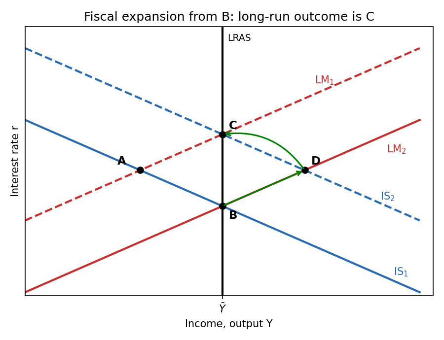
B to D is the short-run effect of the IS shift. D to C is the long-run correction as rising prices shift LM left. Output ends at the same , with higher and .
Why the wrong options fail
- B and C say output rises. In the long run output is pinned at by LRAS.
- D says nothing changes, but and are both higher at C than at B.
🗣️ In plain EnglishExtra government spending gives a short boost, but the economy is already at full capacity in the long run, so the boost gets eaten up by higher prices. Output ends up where it started.
Q16 — How monetary policy works in a small open economy
In a small open economy, the ability to stimulate the economy via monetary policy is enabled through
- A. lowering the interest rate, which increases investments
- B. devaluating domestic currency, which increases net export
- C. appreciating domestic currency, which increases net export
- D. affecting consumption preferences of households
AI-written answer, not official. Check before relying on it.
Answer: B (confidence: high)
Under floating rates a small open economy has , so monetary policy cannot move the interest rate. Instead, expanding shifts right, the currency depreciates (lower ), net exports rise, and increases. See Lec_09-The Open Economy Revisited & Mundell-Fleming Model.
Why the wrong options fail
- A is the closed-economy channel. In a small open economy is pinned at .
- C a monetary expansion depreciates the currency, and an appreciation would lower net exports.
- D monetary policy does not work through consumption preferences.
🗣️ In plain EnglishA small economy can't move its own interest rate, so printing money works by making the currency weaker. That makes exports cheaper and lifts demand.
Q17 — Fiscal expansion under a fixed exchange rate
In a small open economy with a fixed exchange rate, if the government adopts an expansionary fiscal policy, in the new short-run equilibrium:
- A. income and the exchange rate will both rise
- B. the exchange rate will rise, but income will remain unchanged
- C. income will rise, but the exchange rate will remain unchanged
- D. both income and the interest rate will rise
AI-written answer, not official. Check before relying on it.
Answer: C (confidence: high)
shifts right, which would push the exchange rate up. To hold the peg the central bank must buy foreign currency and sell domestic currency, which increases and shifts right. The exchange rate stays at its fixed level and income rises (fiscal policy is effective under a peg). In Lec_09-The Open Economy Revisited & Mundell-Fleming Model: .
Why the wrong options fail
- A and B have the exchange rate moving. A peg means it cannot.
- B also has income flat, the floating-rate result for fiscal policy.
- D the interest rate is tied to in a small open economy.
🗣️ In plain EnglishWith a peg, the central bank has to soak up the pressure on the currency, which ends up giving the economy extra money too. So government spending works at full strength, and the exchange rate doesn't move.
Q18 — Solving a floating-rate Mundell-Fleming model
The LM curve for a small open economy with a floating exchange rate is , and the IS curve is . is in percentage terms (so gives ). , where is the nominal exchange rate. , , , , and the government runs a balanced budget. How many units of domestic output can one unit of foreign currency buy?
- A. 1
- B. 2
- C. 3
- D. 4
AI-written answer, not official. Check before relying on it. Confidence is medium-high: the arithmetic is firm, but the final step depends on the units convention for (see below).
Answer: C, 3 (confidence: medium-high)
Step 1: interest rate. Small open economy, so , hence .
Step 2: income from LM.
Step 3: net exports from IS. Balanced budget so :
Step 4: exchange rate.
Step 5: interpret. In this course is the nominal exchange rate in units of foreign currency per unit of domestic currency (Lec_09-The Open Economy Revisited & Mundell-Fleming Model). So one unit of domestic currency buys of a foreign unit, and one unit of foreign currency buys units of domestic currency. With , that is 3 units of domestic output.
Check in Python
NX = 500/3 = 166.667,e = (200 - 166.667)/100 = 0.3333,1/e = 3.0. Option C.
Why the wrong options fail
- A, B, D (1, 2, 4) do not come from any consistent step. Note that itself is not an option: the question asks for the inverse, .
🗣️ In plain EnglishPin down interest rate, then income, then net exports, and the exchange rate drops out as . The question wants it the other way up, so one foreign unit buys 3 domestic ones.
Q19 — Expected depreciation and today's exchange rate
In the Mundell-Fleming model, expectations that a currency will lose value in the future will cause the current exchange rate to:
- A. increase in the present
- B. decrease in the present
- C. remain constant in the present
- D. decrease only in the future
AI-written answer, not official. Check before relying on it.
Answer: B (confidence: high)
If investors expect the currency to weaken, holding it is less attractive. They sell it now, which lowers its value today. Equivalent in the model: expected depreciation acts like a rise in the country risk premium, shifting left and the exchange rate down. See Lec_09-The Open Economy Revisited & Mundell-Fleming Model.
Why the wrong options fail
- A has it backwards.
- C ignores that expectations move exchange rates immediately.
- D exchange rates are forward-looking asset prices, so the adjustment happens today, not just later.
🗣️ In plain EnglishIf everyone thinks a currency will be worth less soon, they dump it now, and it falls today.
Q20 — Monetary expansion in a large open economy
In a short-run model of a large open economy with a floating exchange rate, a monetary expansion causes a decrease in the interest rate and:
- A. the exchange rate but has no effect on income
- B. the exchange rate, and increases in income, net capital outflow, and net exports
- C. the exchange rate and net capital outflow, and increases in income and net exports
- D. net exports and net capital outflow, but increases in investment and income
AI-written answer, not official. Check before relying on it.
Answer: B (confidence: medium-high)
Reading the stem as "a decrease in the interest rate and [a decrease in] ..." the large open economy chain is:
- shifts right, so the interest rate falls.
- Lower raises net capital outflow (, since domestic assets pay less), so the supply of domestic currency rises and the exchange rate falls.
- Lower makes exports cheaper, so net exports rise.
- Higher investment and net exports raise income .
So the exchange rate falls, while income, net capital outflow and net exports all rise.
Why the wrong options fail
- A says no effect on income. Income rises.
- C puts net capital outflow among the things that decrease. It increases when falls.
- D has net exports falling. They rise when the currency depreciates. It also drops the exchange rate effect.
🗣️ In plain EnglishLower interest rates send money abroad, which makes the currency weaker. A weaker currency boosts exports, so income goes up.
Q21 — A fall in consumer confidence under floating rates
A fall in consumer confidence about the future, which induces consumers to spend less and save more, will, according to the Mundell-Fleming model with floating exchange rates, lead to
- A. a fall in consumption and income
- B. no change in consumption or income
- C. no change in income but a rise in net exports
- D. no change in income or net exports
AI-written answer, not official. Check before relying on it.
Answer: C (confidence: high)
Lower consumption shifts left. Under floating rates is vertical (income set by and ), so income cannot change. Instead the exchange rate falls, which raises net exports. The fall in is exactly offset by the rise in . Income is unchanged.
Why the wrong options fail
- A income does not fall: the exchange rate absorbs the shock.
- B consumption does fall, since that is the shock itself.
- D the currency depreciation raises net exports.
🗣️ In plain EnglishPeople spend less at home, but the currency weakens, so exports pick up the slack. Total income stays put.
Q22 — What drives the slope of the sticky-price AS curve
According to the sticky-price model, the slope of the AS curve in the short run will positively depends on the
- A. fraction of fixed price firms
- B. fraction of flexible-price firms
- C. excess output, above its normal level
- D. price expectation
AI-written answer, not official. Check before relying on it.
Answer: B (confidence: medium-high)
With a fraction of sticky-price firms and flexible-price firms (Lec_14-Aggregate Supply & the Phillips Curve):
The slope rises with the share of flexible firms (and falls with the sticky share ). In the limit of all prices flexible () the curve is vertical.
Why the wrong options fail
- A is the opposite: more sticky firms flatten the curve.
- C is the variable you move along the curve, not what sets its slope.
- D the expected price shifts the curve, not its slope.
🗣️ In plain EnglishThe more firms that can change prices quickly, the more any boost to demand shows up as higher prices rather than more output, so the supply curve gets steeper.
Q23 — Which policy is more inflationary at the same output gain
Consider the AD-AS with upward sloping supply. Assuming that a monetary policy and fiscal policy lead exactly to the same output increase in the short-run, which one would be more inflationary?
- A. Both policies would be equally inflationary
- B. Fiscal policy
- C. Monetary policy
- D. None of the policies will be inflationary
AI-written answer, not official. Check before relying on it.
Answer: A (confidence: medium-high)
Both policies work by shifting AD to the right. If they produce the same output rise along the same SRAS curve, they land on the same point on that curve, so the price level rise is the same. The difference between them (what happens to , and ) does not change where on SRAS the economy ends up.
Why the wrong options fail
- B and C need the two policies to reach different points on the same SRAS curve, which is impossible if output is the same.
- D with upward-sloping SRAS any AD expansion raises .
🗣️ In plain EnglishThe supply curve alone decides how much of a given output boost turns into higher prices. If both policies give the same output, they give the same inflation.
Q24 — Hysteresis: normal unemployment in period 3
The economy is in long-run equilibrium with . Normal unemployment displays hysteresis: . The short-run Phillips curve is . The Fed lowers inflation by 2 points in period 1, then keeps inflation permanently at its new level. If the Fed does what is needed from period 1 on, the normal unemployment rate in period 3 is:
- A. 4
- B. 9
- C. 6.5
- D. 7.75
AI-written answer, not official. Check before relying on it.
Answer: D, 7.75 (confidence: high)
Start with .
Period 1 (inflation falls by 2): , so . , hence .
Period 2 (inflation unchanged): , so . , hence .
Period 3 (inflation unchanged): .
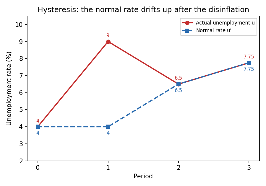
The 2-point disinflation costs 9% unemployment in period 1. Hysteresis then drags the normal rate up from 4 to 6.5 to 7.75.
Why the wrong options fail
- A (4) ignores hysteresis: the normal rate would stay put only if the economy never deviated.
- B (9) is actual unemployment in period 1, not the normal rate in period 3.
- C (6.5) is the normal rate in period 2. Period 3 needs one more averaging step.
🗣️ In plain EnglishBeating inflation costs a deep slump first (9% unemployment). Because the "normal" rate follows past unemployment, it ratchets up too, to 7.75% by period 3, and doesn't come back on its own.
Q25 — Cyclical unemployment needed to cut inflation by 5 points
Assume the Phillips curve . How many percentage points of cyclical unemployment are needed to reduce inflation by 5 percentage points?
- A. 20
- B. 10
- C. 5
- D. 2.5
AI-written answer, not official. Check before relying on it.
Answer: B, 10 (confidence: high)
Cyclical unemployment is . The change in inflation is . Setting this to percentage points (with and in the same units, percentage points):
Ten points of cyclical unemployment: the coefficient 0.5 means each point of unemployment cuts inflation by only half a point.
Why the wrong options fail
- A (20) multiplies by the coefficient instead of dividing.
- C (5) ignores the 0.5 and equates the two changes one for one.
- D (2.5) multiplies .
🗣️ In plain EnglishEach extra point of unemployment only shaves half a point off inflation, so to cut inflation by 5 points you need 10 points of extra unemployment. Painful.
Recap table
| Q | Topic | Answer | Confidence |
|---|---|---|---|
| 1 | Classical loanable funds | B: clears both markets, unaffected | High |
| 2 | Quantity theory, rising velocity | A: inflation increasing | High |
| 3 | Saving tax break, lower | B: necessarily falls | High |
| 4 | Announced vs actual | C: both raise current prices | Med-high |
| 5 | Golden-rule saving rate | B: | High |
| 6 | Steady-state growth per worker | A: zero | High |
| 7 | Persistent growth | D: technological progress | High |
| 8 | Factor price growth | C: wage , rental price 0 | High |
| 9 | Capital and permanent growth | C: false, diminishing returns | Medium |
| 10 | Velocity fall, two central banks | A: both raise | Med-high |
| 11 | Keynesian cross at | A (= B): inventory build-up | High |
| 12 | LM slope | C: bond sales, excess money demand | High |
| 13 | Money to output, closed economy | B: interest rate and investment | Med-high |
| 14 | IS-LM numbers | C: +50, -0.5 | High |
| 15 | Fiscal expansion, long run | A: prices up, output unchanged | Medium |
| 16 | Monetary policy, small open | B: depreciation raises NX | High |
| 17 | Fiscal policy, fixed rate | C: up, unchanged | High |
| 18 | M-F calculation | C: , so | Med-high |
| 19 | Expected depreciation | B: falls now | High |
| 20 | Monetary expansion, large open | B: down; , NCO, NX up | Med-high |
| 21 | Consumer confidence, floating | C: flat, NX up | High |
| 22 | Sticky-price slope | B: share of flexible firms | Med-high |
| 23 | Monetary vs fiscal inflation | A: equally | Med-high |
| 24 | Hysteresis | D: 7.75 | High |
| 25 | Phillips curve | B: 10 points | High |
Related notes
- Hub: Macro-Economics II
- Lec_03-Classical Theory & National Income, Lec_05-Inflation, Lec_06-AS-AD Model & Economic Fluctuations, Lec_07-Aggregate Demand I & the IS-LM Model, Lec_08-Aggregate Demand II & Applying the IS-LM Model, Lec_09-The Open Economy Revisited & Mundell-Fleming Model, Lec_14-Aggregate Supply & the Phillips Curve