
True-False, Price Controls, Production Economy & Externality (2026 Moed A)
- #microeconomics
- #past-paper
- #worked-solution
- #true-false
- #price-controls
- #production-economy
- #externalities
- #pigouvian-tax
True-False, Price Controls, Production Economy & Externality (2026 Moed A)
Part of: Micro-Economics II Micro 2 Final Exam, Moed A (2026), Micro-Economics II. Four questions: Q1 is five true/false items, Q2 a price-control market, Q3 a production economy, Q4 an externality between two exporters. Builds on: Lec_04-Theory of the Firm, Partial & General Equilibrium, Lec_05-Production Economy & Externalities, Lec_06-Public Goods & Altruism Practice: PS_03-Cost Minimisation & Properties of the Cost Function, PS_04-Partial Equilibrium, Welfare & Price Ceilings, PS_05-Pareto Efficiency, Dominance & Social Welfare, PS_06-Exchange Equilibrium, Walrasian Prices & the Social Planner, PS_08-Production Economy, Efficiency Locus & Input Allocation
Question text reconstructedThere is no original question paper for this sitting. The wording of every question below is rebuilt from how the official solution slides restate it (the "Solution Moed A - 2026" deck, 36 slides). Mark allocations are not given anywhere in the deck, so none are shown. Where the deck does not make the full question clear, a
> [!todo] Original wording unknowncallout says so. No givens have been invented.
SourceAnswers follow the official solution. Where the official text has a typo or a gap the answer is kept and a
> [!warning]callout flags it.
What this paper tests
| Question | Core idea | Where it is taught |
|---|---|---|
| Q1 | Five true/false claims: Pareto Dominance vs a planner's choice, marginal cost with a convex technology, cost minimisation with quasi-linear technology, the Contract Curve, and the public-good Nash equilibrium | PS_05-Pareto Efficiency, Dominance & Social Welfare, PS_03-Cost Minimisation & Properties of the Cost Function, Lec_06-Public Goods & Altruism |
| Q2 | Partial Equilibrium with quasi-linear demand and a Cobb-Douglas firm; a government that weights Consumer Surplus and Firm Surplus and chooses a price ceiling or floor | PS_04-Partial Equilibrium, Welfare & Price Ceilings |
| Q3 | Production Economy with a productivity parameter : PPF, RPT vs MRS, equilibrium prices, comparative statics | Lec_05-Production Economy & Externalities, PS_08-Production Economy, Efficiency Locus & Input Allocation |
| Q4 | A two-firm Externalities game: equilibrium vs social planner, and the Pigouvian Tax | Lec_05-Production Economy & Externalities |
Intuition: the one move behind each question
- Q1: for each claim, find one concrete counterexample (false) or run one short derivation (true).
- Q2: price equals marginal cost on the supply side, marginal utility on the demand side; a binding control makes the short side decide the quantity.
- Q3: equalise RTS across firms to get a straight-line PPF with slope ; then price ratio = RPT = MRS.
- Q4: each firm's effort is free to itself but costs the rival 4 per unit, so the market overuses effort.
Q1 — True or false (five items)
Original wording unknownThe deck restates each claim as a statement to be judged true or false. The instruction line for the section (for example "determine whether each claim is true or false and explain") and the marks per item are not shown. The five claims below are quoted from the slides.
Q1.1 — Adding a feasible alternative
Claim. Consider a social planner who faces a set of alternatives and chooses alternative . Suppose now that an additional alternative is added to the feasible set, after which the social planner chooses . Alternative Pareto dominates alternative .
AnswerFalse.
Counterexample (official). Exchange economy with , and endowments . The planner's welfare is
The contract curve is .
| Allocation | Agent 1 gets | Agent 2 gets | |||
|---|---|---|---|---|---|
The planner prefers to ( against ), yet does not Pareto dominate : agent 1 gains () but agent 2 loses ().
IntuitionA welfare function can trade one person's loss against another's gain. "The planner prefers " only means the weighted total went up. Pareto Dominance needs nobody worse off. Preferred by is much weaker than dominating.
Typo in the official solutionThe last line says " doesn't dominate allocation b". There is no allocation in the question; it means allocation .
Q1.2 — Convex production with one input
Claim. Consider a firm that produces using a single input, labour. Assume that the production function is increasing and strictly convex. Then the marginal cost of production is increasing.
AnswerFalse. Marginal cost is decreasing.
Why (official). With one input, , so
If is convex, is increasing in , so is decreasing in . Since rises with , is decreasing in .
IntuitionConvex means each extra hour of labour adds more output than the last (increasing returns). So each extra unit of output needs less extra labour, and costs less at the margin. Marginal cost rising is the concave story (diminishing marginal product). To make the claim true you would need concave.
Q1.3 — Quasi-linear technology
Claim. Consider a firm whose production function is quasi-linear, , where is a concave function. Suppose that . Then, at any output level, an increase in the firm's production level does not lead to an increase in the use of input .
AnswerFalse.
Why (official). The firm minimises cost, which depends on input prices as well as marginal products. If there is an with
then the firm uses labour and raises its labour for output levels . For example, when labour is sufficiently cheap relative to capital, labour delivers more output per unit of cost than capital, so the cost-minimising choice uses positive labour and, as rises, the firm increases .
Intuitionis concave, so falls as rises. At low output the firm uses only labour (while , labour is the better buy per dollar) and rises with . Once reaches the point where , extra output comes from capital, which has a constant marginal product of , so stops growing. The claim says "at any output level", so one range where rises is enough to make it false. The condition is compatible with this as long as is small enough, which is what "labour sufficiently cheap relative to capital" means.
Q1.4 — The midpoint allocation
Claim. Consider an exchange economy with two agents. The agents' utility functions are and , where and . The aggregate endowments of goods and are and . Then the allocation is not on the contract curve.
AnswerTrue.
Why (official). A point on the contract curve must be Pareto efficient, so :
At the midpoint each agent gets half of everything: and . The common factor cancels, so equality would need
Since , the MRS values differ, the allocation is not Pareto efficient and so is not on the contract curve.
IntuitionWith the same bundle each, the agent with the larger Cobb-Douglas weight on values more at the margin. They would both gain from trading, so the midpoint cannot be efficient. It lies on the contract curve only in the knife-edge case (compare PS_06-Exchange Equilibrium, Walrasian Prices & the Social Planner).
Q1.5 — Public good game with identical agents
Claim. Consider a two-agent public good game, as studied in class. If the two agents have identical utility functions, then there exists a unique Nash equilibrium in which both agents contribute the same amount to the public good.
AnswerFalse.
Why (official). When both agents have the same utility function, every combination of and that results in the total quantity is a Nash equilibrium, and there are infinitely many such combinations.
Link to the lecture. In Lec_06-Public Goods & Altruism the best response is . When , any pair with satisfies both best responses. The equal split is one equilibrium among infinitely many, so the equilibrium is neither unique nor forced to be symmetric.
IntuitionEach agent only cares about the total supply of the public good. Once the total hits what both of them want, neither wants to change, no matter who paid for how much of it.
Q2 — Price controls and the government's objective
Setup (as restated in the solution). A market for goods and , where represents money. Demand comes from a representative consumer with utility
(income is high enough that there are no corner solutions). Supply comes from a representative firm with production function
and input prices and .
Questions (as restated in the solution).
- Derive the inverse demand function and the inverse supply function in the market. Provide an economic explanation for the derivation.
- Find the equilibrium price and the equilibrium quantity in the market.
- Calculate the overall welfare in equilibrium, the consumer surplus, and the firm surplus.
The government can now intervene by setting a maximal price or a minimal price for the good . Its objective is , where is consumer surplus and is firm surplus.
- Assume . Find the government's optimal policy.
- Assume and . Find the government's optimal policy.
- Assume and . Find the government's optimal policy.
- Assume . Find the set of policies that cannot be optimal.
- Assume . Find the set of policies that cannot be optimal.
Q2.1 — Inverse demand and inverse supply
Answer
Demand. The utility is quasi-linear with as money (price ), so the consumer's price equals the marginal utility of : . The consumer buys until the last unit is worth exactly its price.
Supply. The firm's supply is its marginal cost, so first find the cost function.
- Cost minimisation: , so .
- Put this into the isoquant for output : , hence .
- Cost: .
- Supply: .
Why. A price-taking firm produces until price equals marginal cost, so the MC curve is the supply curve. The consumer's marginal utility is the maximum they will pay for one more unit, so it is the demand curve.
Q2.2 — Equilibrium
Answer,
Set , so and .
Q2.3 — Welfare, consumer surplus, firm surplus
AnswerTotal welfare , consumer surplus , firm surplus .
Total welfare is the area between marginal utility and marginal cost:
Consumer surplus is the area between demand and the price line:
Firm surplus is the area between the price line and supply:
Check: .
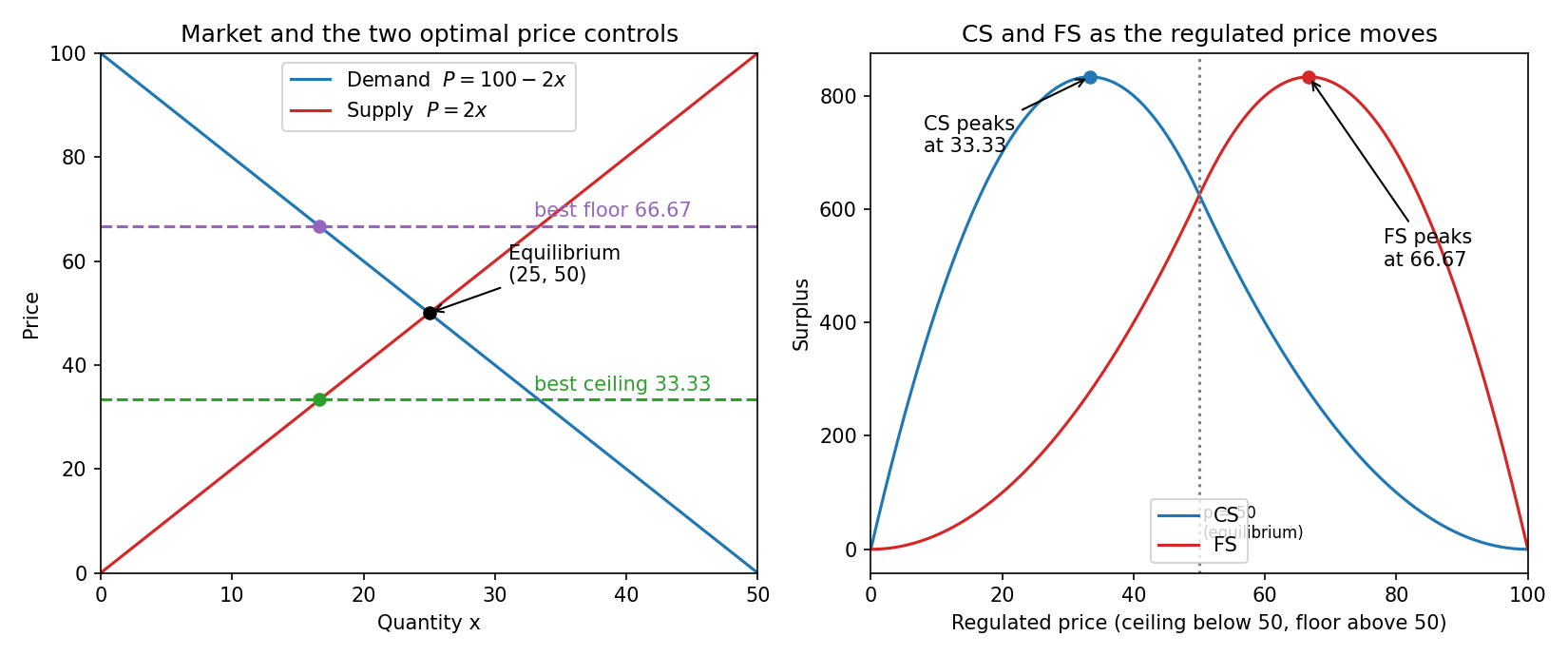
Left: demand, supply and the two best price controls found in parts 5 and 6. Right: how consumer surplus (CS) and firm surplus (FS) move as the regulated price moves away from . The ceiling is a price below , the floor a price above .
Q2.4 — Equal weights,
AnswerTotal surplus is maximised at the competitive equilibrium, price . The government can do nothing, set a maximal price , or set a minimal price . All of these leave the equilibrium in place and maximise its objective.
With the objective is , a multiple of total surplus. Any binding control moves the quantity away from and loses surplus. Non-binding controls (a ceiling at or above , a floor at or below ) change nothing.
Q2.5 — Only consumers matter, ,
AnswerSet a maximal price at .
The government only cares about .
- A price floor above lowers CS, so it cannot help. The only useful tool is a ceiling below .
- With a binding ceiling , the quantity is set by supply (the short side): .
- Consumer surplus:
- First-order condition:
IntuitionA lower ceiling gives consumers a cheaper price but cuts the quantity they can buy. Near the price gain beats the quantity loss, so the ceiling helps. Below the lost quantity wins. CS peaks at (in the figure, the blue curve on the right).
Q2.6 — Only firms matter, ,
AnswerSet a minimal price at .
The government only cares about .
- A price ceiling below lowers FS, so the only useful tool is a floor above .
- With a binding floor , the quantity is set by demand (the short side): .
- Firm surplus:
- First-order condition:
Q2.7 — Consumers weighted more,
AnswerPolicies that cannot be optimal: any price floor , and any price ceiling .
Why (official). Consumers count more than firms. Any floor at or above cannot be optimal. A ceiling below raises CS until the price reaches , the CS maximum; a lower ceiling reduces both CS and FS, so it is worse.
Intuition: check with the derivative (my own check)Using the surplus formulas above, the objective along a floor has slope , which at equals when : raising the price above already hurts the government. Along a ceiling, and the slope is . At this is , so the objective is still rising there and is increasing for all lower prices too. Ceilings below are therefore beaten by a ceiling at . This also shows the equilibrium itself (, or a non-binding ceiling) is not optimal here.
Q2.8 — Firms weighted more,
AnswerPolicies that cannot be optimal: any price ceiling , and any price floor .
Why (official). Firms count more than consumers. Any ceiling at or below cannot be optimal. A floor above raises FS until the price reaches , the FS maximum; a higher floor reduces both FS and CS, so it is worse.
Typos in the official solutionThe text says "producers are weighted more than firms" in Q2.8 and "consumes surplus increases until price reaches maximum" in Q2.7. These are slips ("firms" should be "consumers" in Q2.8). The answers are unaffected. The slide writes ; the exact value is .
Q3 — A production economy with a productivity parameter
Setup (as restated in the solution). A production economy with two firms:
The representative consumer has utility . The resource constraints are and . Firm 1 produces and firm 2 produces .
Original wording unknownThe deck does not say which good each firm produces. It is clear from the working that and ("", ""), so that is used here.
Questions (as restated in the solution).
- How does social welfare change as changes? Base your answer on an analysis of the environment (an intuitive explanation is not sufficient).
- Assume and . Find the equilibrium allocation and the equilibrium prices.
- Consider an arbitrary economy with the above structure (no specific values for the parameters other than those given at the start).
- a. How does the equilibrium price ratio change as changes? (Hint: you do not necessarily need a full analysis of the equilibrium to give a logical answer.)
- b. How does the equilibrium quantity ratio change as changes?
Q3.1 — Social welfare as rises
AnswerSocial welfare increases with .
Step 1: efficient input allocation. Compute the RTS of each firm. For firm 1, and , so
The factor cancels in the ratio. Efficiency needs , so
Step 2: outputs. With (and ):
Step 3: the PPF. Eliminating (so ):
The PPF is a straight line, so everywhere.
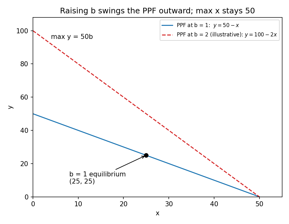
The PPF is a straight line from to . A higher raises the -intercept and keeps the -intercept at . The line is only illustrative; the point is the equilibrium from Q3.2.
Step 4: conclusion. As rises, the maximum that can be produced, , rises while the maximum stays . The PPF moves outward at every , so the consumer can reach strictly more for any .
Intuition: why this is a proof and not just a storyBecause is increasing in , the bundle that was optimal at the old is still feasible at the new, larger , and the same with more is strictly better. So the welfare maximum can only go up. (This last sentence is my own filling-in of the argument.)
Q3.2 — Equilibrium for ,
Answerand . Prices: (taking ) and .
Allocation.
- With the PPF is , so .
- With , .
- Set : .
- Combine with the PPF: . From and the efficiency condition : , and then .
Prices.
- Output prices: , with as the numeraire ().
- Input prices: firm 1's RTS equals the input price ratio, , so . Here .
- To pin down the level, derive firm 1's cost function. Substitute into :
- Profit maximisation (price equals marginal cost): .
- With : , so .
Note on the official workingThe slide's cost-function steps use , which means firm 1's exponent is . The question as restated fixes and but not , so the official solution silently takes here. The allocation does not depend on (the efficiency condition holds for every ), but the input prices above do.
Q3.3a — Price ratio as changes
Answer, so the price ratio increases with .
As rises, the slope of the PPF rises. The PPF is a straight line, so it coincides with the consumer's budget line in equilibrium (the budget line has slope ). Hence in the optimal bundle .
IntuitionProducing one more unit of costs units of (the RPT). A competitive price ratio must reflect this opportunity cost, so becomes relatively more expensive as gets easier to make.
Q3.3b — Quantity ratio as changes
Answerdecreases with .
At the optimum . For the slide writes , so falls as rises. A higher means the economy can turn resources into more effectively, so the PPF is steeper. The consumer faces what looks like a fall in the price of (with no change in income), and Cobb-Douglas preferences shift the consumption mix towards , so falls.
Intuition (my own generalisation to any )For the MRS is , so setting it equal to gives . This is decreasing in for every , which agrees with the official conclusion.
Q4 — Two exporters and an effort externality
Setup (as restated in the solution). A market where two firms, and , export a given product abroad. The international price is . The cost function of firm is
and of firm :
Original wording unknownThe deck does not say what and stand for (the "effort" label is used below only as a convenient name; the official explanation itself says each firm's "effort" benefits itself and harms the other). The slide itself uses for the price firm receives; it is the international price, .
Questions (as restated in the solution).
- (a) Find the equilibrium in this market (an equilibrium is a choice of for firm and a choice of for firm ) and each firm's profit in equilibrium.
- (b) Assume now that a social planner, whose aim is to maximise the sum of the firms' profits, decides on the quantities .
- (i) Find the optimal quantities for the social planner, and each firm's profit under the planner's optimal quantities.
- (ii) What happens to the quantity of good that each firm produces compared with the equilibrium level? On the other hand, what happens to each firm's profit compared with its profit in equilibrium? Provide an economic explanation for this seemingly puzzling result.
- (c) Find the Pigouvian tax in this setting.
Q4a — Equilibrium
Answer, and .
Firm 's profit is
- Choose . Firm treats as given (the term is a constant to it). The term is a pure cost to , and affects nothing else in 's own profit. So sets to make it vanish.
- Choose . With : , so .
- By symmetry .
- Profit. . By symmetry .
Q4b(i) — The planner's optimum
Answer, , and each firm's profit is .
The planner maximises total profit:
- Effort . Now appears in 's own cost term and in 's cost ():
- Quantity .
- By symmetry , .
- Profit. . By symmetry .
Q4b(ii) — Why less output but higher profit?
AnswerEach firm produces less ( against ) but earns more ( against ).
Why (official). Each firm's effort benefits itself but harms the other by raising the other firm's cost. In equilibrium firms ignore this and overuse effort. The planner internalises the externality, reduces both effort and output, and achieves higher overall efficiency and profit.
IntuitionThis is the classic mutual negative externality. Each firm gets a private benefit from effort (it cancels its own adjustment cost ) while the cost of per unit lands on the rival. The market is a prisoners' dilemma: both would be better off if both cut effort, but neither has a private reason to. Cutting effort from to and output from to raises profit from to each, a joint gain of ( against ).
Q4c — Pigouvian tax
AnswerThe Pigouvian tax is 4 (per unit of ).
One extra unit of raises firm 's cost by , and one extra unit of raises firm 's cost by . A Pigouvian Tax equals the marginal external damage of the action. Here the external damage from is constant and equals , so the tax is .
Intuition: check against Q4b (my own check)With a tax of on , firm 's profit becomes . Its first-order conditions are (from ) and (from ), which are exactly the planner's conditions, giving and . So a tax of implements the planner's optimum.
Recap table
| Part | Tool | Answer |
|---|---|---|
| Q1.1 | Welfare preference is not Pareto dominance | False (: , but agent 2 falls ) |
| Q1.2 | with rising | False, MC decreasing |
| Q1.3 | Cost minimisation with | False, rises at low output |
| Q1.4 | at the midpoint | True () |
| Q1.5 | Public good Nash equilibrium | False, infinitely many with |
| Q2.1 | MU = demand, MC = supply | , |
| Q2.2 | , | |
| Q2.3 | Areas under demand and supply | , |
| Q2.4 | means total surplus | No control, or non-binding ones |
| Q2.5 | Maximise CS under a ceiling | Ceiling at |
| Q2.6 | Maximise FS under a floor | Floor at |
| Q2.7 | Not optimal: floors , ceilings | |
| Q2.8 | Not optimal: ceilings , floors | |
| Q3.1 | , PPF | Welfare rises with |
| Q3.2 | , | , all inputs , |
| Q3.3a | PPF coincides with budget line | , rises |
| Q3.3b | falls | |
| Q4a | , | , each |
| Q4b(i) | Maximise joint profit | , , each |
| Q4b(ii) | Internalise the externality | Less output, more profit |
| Q4c | Marginal external damage | Tax |
Related notes
- Micro-Economics II (hub)
- Lec_04-Theory of the Firm, Partial & General Equilibrium
- Lec_05-Production Economy & Externalities
- Lec_06-Public Goods & Altruism
- PS_03-Cost Minimisation & Properties of the Cost Function
- PS_04-Partial Equilibrium, Welfare & Price Ceilings
- PS_05-Pareto Efficiency, Dominance & Social Welfare
- PS_06-Exchange Equilibrium, Walrasian Prices & the Social Planner
- PS_08-Production Economy, Efficiency Locus & Input Allocation