
Perfect Substitutes, Exchange Equilibrium, Minimum Price & Social Planner (2024 Moed A)
- #microeconomics
- #past-paper
- #worked-solution
- #perfect-substitutes
- #cost-function
- #exchange-economy
- #contract-curve
- #minimum-price
- #social-planner
Perfect Substitutes, Exchange Equilibrium, Minimum Price & Social Planner (2024 Moed A)
Part of: Micro-Economics II Micro 2 Final Exam, Moed A (March 2024), Micro-Economics II, Dr. Boaz Zik. 3 hours, open material, 4 questions, 25 points each. Builds on: Lec_04-Theory of the Firm, Partial & General Equilibrium, Lec_05-Production Economy & Externalities Practice: PS_03-Cost Minimisation & Properties of the Cost Function, PS_04-Partial Equilibrium, Welfare & Price Ceilings, PS_06-Exchange Equilibrium, Walrasian Prices & the Social Planner, PS_07-Core, Corner Endowments & Equilibrium vs the Social Planner
SourceAnswers follow the official solution (12 pages). Where the official text has a typo or a gap, the answer is kept and a
> [!warning]callout flags it.
What this paper tests
| Question | Core idea | Where it is taught |
|---|---|---|
| Q1 | Perfect Substitutes technology: linear isoquants, corner cost minimisation, flat supply, zero profit | PS_03-Cost Minimisation & Properties of the Cost Function, Lec_04-Theory of the Firm, Partial & General Equilibrium |
| Q2 | Exchange Economy with Cobb-Douglas agents: Contract Curve, Walrasian Equilibrium, what the shape of the contract curve says about preferences | PS_06-Exchange Equilibrium, Walrasian Prices & the Social Planner |
| Q3 | Partial Equilibrium with quasilinear demand and a minimum price (price floor): how Consumer Surplus and Firm Surplus move with the floor, increasing vs constant marginal cost | PS_04-Partial Equilibrium, Welfare & Price Ceilings |
| Q4 | Contract curve, utility frontier and a Cobb-Douglas social planner | PS_05-Pareto Efficiency, Dominance & Social Welfare, PS_07-Core, Corner Endowments & Equilibrium vs the Social Planner |
Intuition: the one move behind each question
- Q1: with perfect substitutes the firm just uses whichever input gives more output per dollar, so the answer is always a corner (or a tie).
- Q2 and Q4: find the contract curve by setting and substituting the resource constraints.
- Q3: price = marginal cost on the supply side, price = marginal utility on the demand side. A floor above equilibrium means the short side of the market (demand) decides the quantity.
Q1 — Perfect substitutes technology (25 points)
Production function .
1a — Quantity at a convex combination of two isoquant points (7 points)
Question. Take two bundles and on the same isoquant and with . How does the quantity under compare with the quantity under and ? Prove it.
Answerproduces exactly the same quantity as and .
Proof (official). Let and both produce :
By definition of :
Substituting the two isoquant equations into :
So lies on the same line , hence produces .
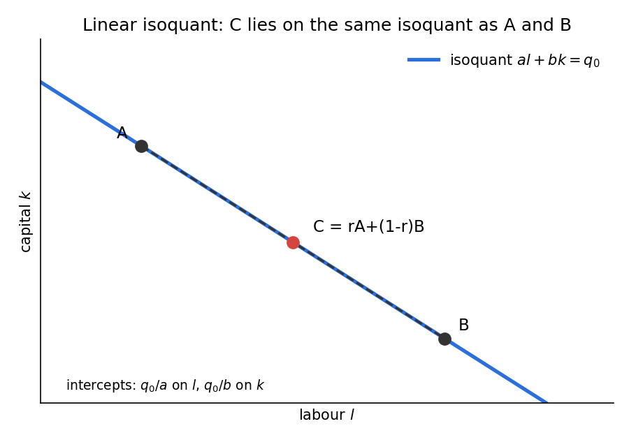
The isoquant is a straight line, so every point between and stays on it.
IntuitionThis is the knife-edge case of the convex isoquant property from PS_02-Isoquants, RTS & Properties of the Profit Function. For a strictly convex isoquant (Cobb-Douglas), the midpoint of and lies on a higher isoquant. For perfect substitutes the isoquant is flat-straight, so the midpoint is on the same one: there is no gain from "mixing" inputs. That is exactly why the cost-minimiser ends up at a corner.
1b — Cost function when (6 points)
Answer, , so
Why. The condition is the same as : labour gives more output per dollar than capital. The RTS is the constant (slope of the isoquant) and the isocost slope is . Since the isoquant is steeper than the isocost line, the isocost line touches the isoquant only at the labour-axis corner. The firm uses labour only: .
1c — A fall in (6 points)
Question. What happens to the chosen and to when falls?
AnswerIt depends on where ends up relative to (a fall in raises ):
After the fall Regime still labour corner stays unchanged, indifferent anywhere from to unchanged, capital corner jumps to changes to
Why. The firm is bang-bang: small price changes do nothing while the same input stays cheaper per unit of output, and the firm switches entirely once the ranking flips. In the third case the new cost is below the old (that is what means), so cost falls.
1d — Supply function and equilibrium profit (6 points)
Answer, so the supply (inverse) function is the marginal cost a horizontal line. In equilibrium , so profit per marginal unit is zero for every and the firm makes zero profit.
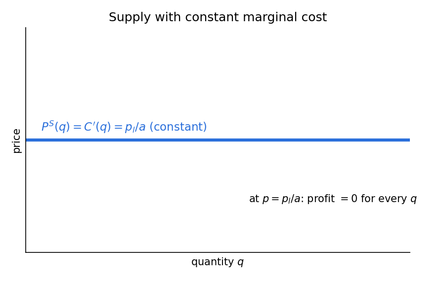
Constant marginal cost gives a perfectly elastic supply curve at height .
IntuitionConstant returns to scale (the cost is linear in ) means no fixed cost and no rising marginal cost to earn a rent on. Competition pushes price to and nothing is left over. This zero-profit result is used again in Q3(g).
Q2 — Exchange economy with Cobb-Douglas agents (25 points)
and , total resources and .
2a — Numerical case: , , ,
(1) Contract curve (5 points)
Answer
The Contract Curve is where .
With and :
Cross-multiplying: , so , giving , the stated curve.
(2) Equilibrium prices and quantities (5 points)
Answer(good is the numeraire), and
Agent 1 maximises subject to . Cobb-Douglas spends the share of income on :
Agent 2 maximises on the same budget form:
Market clearing for ():
Plugging back gives the allocation above. By Walras' Law the market clears automatically.
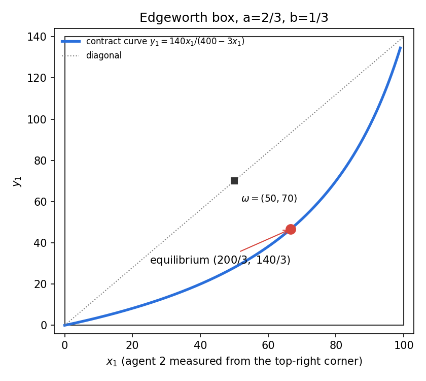
The equilibrium allocation lies on the contract curve, as the First Welfare Theorem requires. Agent 1, who likes more, ends up with more than the endowment.
IntuitionAgent 1 has (loves ), agent 2 has (loves ). Both start with the same bundle, so agent 1 sells and buys . The allocation sits below the diagonal: and .
2b — Contract curve (5 points)
AnswerThis holds if and only if .
Proof (official), both directions.
( line). Equal MRS gives
and with , :
Cross-multiplying: , so .
(line ). If then , so . The contract curve condition then forces , i.e. .
IntuitionIdentical tastes mean that when both agents face the same ratio their MRS is equal. The contract curve is then the Edgeworth box diagonal: efficient allocations give both agents the same bundle proportions.
2c — Price ratio when , diagonal contract curve, (5 points)
Answer
With the diagonal is . A competitive equilibrium in the interior is Pareto efficient, so it sits on the contract curve, and the price ratio equals the MRS:
On the diagonal , so .
2d — Contract curve passes above the centre: (5 points)
Answer, and more precisely .
Why (official). By 2b, if the contract curve is the diagonal and passes through the centre . A curve strictly above the centre therefore means . At the point where is split evenly, agent 1 gets more than agent 2, so agent 1 values more relative to : .
Intuition: check it with the MRSAt : equal MRS requires . If , then must be smaller than , so . The agent who weights more (agent 1) gets more when is split equally.
Q3 — Partial equilibrium and a minimum price (25 points: parts 3, 3, 7, 3, 3, 3, 3)
Demand comes from a consumer with quasilinear utility ( is money). Supply comes from a representative firm.
Setup used in every partFor Quasilinear Utility, the inverse demand is the marginal utility of : . The inverse supply is the marginal cost: . See PS_04-Partial Equilibrium, Welfare & Price Ceilings.
Part I: firm with ,
3a — Cost function (3 points)
Answer
Set RTS equal to the price ratio: , so . The isoquant is , so and
3b — Equilibrium (3 points)
Answer,
. Equate , so and .
3c — Minimum price (7 points)
Question. Find the consumer surplus and the firm's surplus as functions of , and where each is increasing or decreasing.
Answer
- If : the floor does not bind, price is 48 and quantity 6. and firm surplus . Both are constant.
- If : quantity is set by demand, .
- decreases in throughout (down to 0 at ).
- Firm surplus is , which increases until and decreases afterwards.
Derivation. Above the equilibrium price, firms would gladly supply more than consumers want to buy, so the quantity traded is the short side, which is demand: .
Firm surplus:
First-order condition: , so is the peak.
Typo in the official consumer surplusThe solution prints . Computing it: . At this gives , matching the "36" in the first case (with it would be 72, which breaks continuity). The conclusion (decreasing in ) is unaffected. The version is used here.
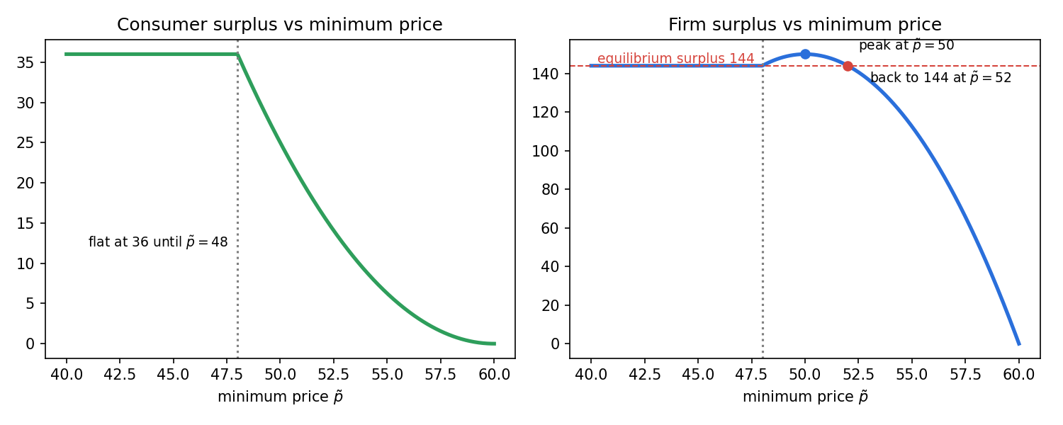
Left: consumer surplus is flat at 36 and then falls once the floor binds. Right: firm surplus rises from 144 to a peak of 150 at , then falls and crosses back through 144 at .
IntuitionA small floor above 48 makes the firm earn more per unit, which outweighs the units lost. Beyond 50 the lost sales dominate. This is the standard price-floor trade-off: the producer benefits from the higher price only while the volume loss is small, because the firm has rising marginal cost so the units lost were not very profitable.
3d — When is the firm worse off than in equilibrium? (3 points)
AnswerFor .
Set firm surplus equal to its equilibrium value, 144:
which has roots and (the official solution reports the positive root 52 that is relevant above 48). Above 52 firm surplus is strictly below 144.
Part II: firm with , ,
3e — Cost function (3 points)
Answer
RTS equals the price ratio: , so . The isoquant gives and . Then
Printed typoThe official text writes the condition as "" in one place but the numbers it then uses (, , ) correspond to , which is the correct tangency above.
3f — Equilibrium (3 points)
Answer,
. Equate , so and .
3g — Minimum price with constant marginal cost (3 points)
AnswerThe firm makes zero surplus in equilibrium, whereas any floor gives it a positive surplus. So the firm never loses from a minimum price, unlike part (d), where a high enough floor leaves it worse off.
Economic explanation. In (d) the firm had increasing marginal cost, so extra production earned a rent, and a high floor that cut the quantity destroyed more rent than the higher price created. Here marginal cost is constant (as in Q1d), so there is no rent from the quantity in equilibrium to lose: the equilibrium surplus is zero, and any floor above 4 can only help.
Gap in the official solutionThe last sentence of the official explanation is cut off ("The explanation for the difference is that when the firm has constant marginal cost."). The reading above is the natural completion. Also, strictly, at demand is zero, so quantity and surplus are , which equals (not exceeds) the equilibrium surplus. The statement "never loses" is therefore weakly true.
Q4 — Exchange economy and the social planner (25 points)
, , .
4a — Contract curve (5 points)
Answer(the diagonal of the box)
and . With , :
Cross-multiplying: , so , i.e. .
IntuitionBoth agents have the same Cobb-Douglas exponents (). The factor 2 in scales the utility level but leaves the MRS unchanged, so it does not move the contract curve. This is the case from Q2(b) with .
4b — The planner's problem (5 points)
Answersubject to and .
This is with the utilities substituted in.
4c — Optimal allocation (10 points)
Answer, , , .
Method (official). This is the same algorithm as the planner in a production economy: first restrict to efficient allocations, then trace the utility frontier, then find the tangency with the planner's indifference curve.
Step 1: utility frontier. On the contract curve :
So the frontier is , a straight line with slope .
Step 2: the planner's MRS. For :
Step 3: tangency. Set , so . Plug into the frontier:
Since : , and . Check: .
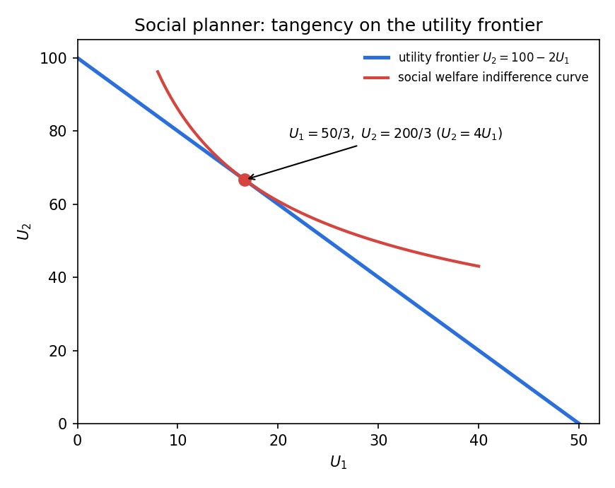
The planner picks the point where the highest social-welfare indifference curve just touches the utility frontier.
IntuitionThe planner weights agent 2 twice as much (exponent vs ), and agent 2's utility is also scaled up by the factor 2. Agent 2 therefore ends up with more of the resources (two thirds of each good) and four times the utility of agent 1.
4d — General weight : (5 points)
Answer (official)The official solution states obtained from , and explains that the planner divides utility according to the weights in its Cobb-Douglas objective: with equal weights () the resources are split equally and agent 2 gets twice the utility; when falls, agent 2 gets more.
Concern: the official formula looks invertedDifferentiating gives (the weight on is in the numerator). Setting this equal to the frontier slope 2 gives Check against part (c): gives , which is the found in 4c. The official formula would give at , contradicting 4c. The corrected form is also what the question seems to be after (ratio of utilities as a function of : proportional, factor 2). It also agrees with the official explanation that a lower gives agent 2 more. The official wording is kept above; check with the lecturer before relying on either form in an exam.
Derivation with the check. The frontier does not depend on the planner's weights, so its slope is for any . Tangency: . Equal weights (): and give , , so and resources are split equally while utilities are (the extra factor 2 in does that). Both versions agree at , which is why the typo is easy to miss.
IntuitionThe weight is how much the planner cares about agent 1. A smaller (larger ) tilts utility, and resources, towards agent 2.
Recap table
| Part | Tool | One-line answer |
|---|---|---|
| 1a | Linear isoquant algebra | is on the same isoquant: same output |
| 1b | Corner solution, | , labour only |
| 1c | Comparative statics on a corner | stays 0, becomes any value up to , or jumps to depending on vs |
| 1d | Flat supply at , zero profit | |
| 2a1 | ||
| 2a2 | Walrasian equilibrium | , |
| 2b | Equal MRS with identical shares | iff contract curve is |
| 2c | Price = MRS on the diagonal | |
| 2d | Curve above the centre | |
| 3a | RTS = price ratio | |
| 3b | , | |
| 3c | Short side of the market | falls, firm surplus peaks at |
| 3d | Solve | Firm worse off for |
| 3e | RTS = price ratio | |
| 3f | , | |
| 3g | Constant MC, zero equilibrium surplus | Firm never loses from a floor |
| 4a | ||
| 4b | Planner's problem | maximise s.t. resource constraints |
| 4c | Utility frontier tangency | , , |
| 4d | Frontier slope = planner MRS | Official (flagged; correct tangency gives ) |
Related notes
- Micro-Economics II (hub)
- Lec_04-Theory of the Firm, Partial & General Equilibrium
- Lec_05-Production Economy & Externalities
- PS_03-Cost Minimisation & Properties of the Cost Function
- PS_04-Partial Equilibrium, Welfare & Price Ceilings
- PS_05-Pareto Efficiency, Dominance & Social Welfare
- PS_06-Exchange Equilibrium, Walrasian Prices & the Social Planner
- PS_07-Core, Corner Endowments & Equilibrium vs the Social Planner