
Corner Solutions, Efficiency Locus, PPF & Fixed Price (2023 Example Exam)
- #microeconomics
- #past-paper
- #worked-solution
- #practice-exam
- #true-false
- #production-economy
- #efficiency-locus
- #ppf
- #partial-equilibrium
- #price-floor
Corner Solutions, Efficiency Locus, PPF & Fixed Price (2023 Example Exam)
Part of: Micro-Economics II Micro 2 Example Final Exam (2023), Micro-Economics II, Dr. Boaz Zik. A practice exam, not a real sitting. 3 hours, cheat sheet and calculator allowed. Part 1 = 10 true/false statements (5 points each), Q2 = 25 points, Q3 = 25 points. Builds on: Lec_04-Theory of the Firm, Partial & General Equilibrium, Lec_05-Production Economy & Externalities Practice: PS_02-Isoquants, RTS & Properties of the Profit Function, PS_03-Cost Minimisation & Properties of the Cost Function, PS_04-Partial Equilibrium, Welfare & Price Ceilings, PS_05-Pareto Efficiency, Dominance & Social Welfare, PS_06-Exchange Equilibrium, Walrasian Prices & the Social Planner, PS_08-Production Economy, Efficiency Locus & Input Allocation
SourceAnswers follow the TA recitation "Micro 2 - 2023, Recitation 12 - Example Exam" (Yosi Ganel, 41 slides). The 2026 version of that recitation was not needed. Where the recitation gives a setup but no explicit verdict, that is flagged and the verdict is completed from its own working.
What this paper tests
Intuition: the one move behind each part
- True/false: for a "necessarily" or "always" claim, one counterexample makes it false. For "the contract curve is a line", go back to .
- Q2: find where the two firms' RTS are equal (efficiency locus), turn it into a PPF, then set .
- Q3: demand is marginal utility, supply is marginal cost; a fixed price above equilibrium means the short side (demand) sets the quantity.
Part 1 — True or false (50 points, 5 points each)
(1) Higher and the same output
Statement. A firm makes from capital and labour. The ratio rises and the firm keeps producing . After the change the firm necessarily uses less labour and more capital.
Answer: False
Why. "Necessarily" fails for a technology with corner solutions. Take (Perfect Substitutes). When rises, the firm can:
- switch from the corner "labour only" to the corner "capital only", or
- stay at the same corner (only , or only ), where usage does not change at all.
So labour does not have to fall and capital does not have to rise.
IntuitionWith smooth (Cobb-Douglas) isoquants a higher does shift the firm towards capital. The statement is only false because the claim covers every technology. See the bang-bang behaviour in PS_03-Cost Minimisation & Properties of the Cost Function.
(2) Agent 2's taste parameter moves from to
Statement. and , resources . Agent 2's utility changes to with . Any interior allocation on the old contract curve is no longer Pareto efficient.
Answer: TrueThe recitation sets up the two contract curves and the check but stops before stating the verdict. The verdict below is completed from its working.
Before the change. gives
Cross-multiplying, : the old contract curve is the diagonal of the Edgeworth Box.
After the change. The condition becomes
Check an old point. Take any interior point on the old diagonal. There , so the common ratio cancels from both sides and the new condition would need
But is strictly increasing in , so gives . The MRS are not equal at the old point, so it is no longer Pareto efficient.
IntuitionThe diagonal was efficient only because both agents had the same tastes. Once agent 2 values relatively more, trade is possible at every interior diagonal point (agent 2 buys from agent 1 for ). The edge points are excluded because there one agent holds nothing of a good and the MRS comparison is not interior.
(3) and
Answer: True
The marginal cost of the very first unit already exceeds the price. Since , marginal cost is rising, so every further unit costs even more. At every positive quantity the firm would make a loss on the margin, so the profit-maximising quantity is 0.
(4) Two exchange economies with vs
Statement. Economy 1: both agents have . Economy 2: both agents have , with . Resources , in both. The contract curve is the same.
Answer: TrueAgain the recitation derives both contract curves, finds them identical, and does not print the word "True".
In economy 1:
In economy 2 the same steps give the same equation, because cancels exactly as did. When the two agents have identical preferences, the contract curve is the box diagonal whatever the parameter is.
Contrast with (2)(4) changes both agents together, so the tastes stay identical and the curve does not move. (2) changes only agent 2, so the tastes diverge and the curve moves.
(5) Representative consumer's rises to : does the PPF shift?
Answer: False
The PPF depends only on technology and resource endowments. The consumer's utility chooses which point on the PPF is produced (the tangency ), but it does not move the frontier itself.
(6) Efficient , inefficient , planner prefers
Statement. If a social planner prefers allocation (Pareto efficient) to (not efficient), then Pareto dominates .
Answer: False
Counterexample (official). , , endowments each, planner welfare . The contract curve is .
| Allocation | , | On contract curve? | |||
|---|---|---|---|---|---|
| , | yes, Pareto efficient | 100 | 100 | 10,000 | |
| , | no (), not efficient | 2 | 342 | 684 |
The planner prefers to (10,000 vs 684), yet agent 2 is worse off at (). So does not Pareto dominate .
IntuitionPareto Dominance needs every agent weakly better off. A planner's score trades one agent's gain against another's loss, so it can rank higher while someone loses. See PS_05-Pareto Efficiency, Dominance & Social Welfare.
(7) , , , output 6
Statement. The firm uses only labour.
Answer: False
Since , labour is relatively too expensive for what it delivers: the firm uses only capital ().
Intuition: output per dollarLabour gives units per dollar, capital gives units per dollar. Capital is the better buy, so the corner is "capital only". This is the same test as vs for perfect substitutes.
(8) Exchange economy with externalities
Statement. The equilibrium is necessarily not Pareto efficient.
Answer: False
Use the whisky and cigars example from the lecture (Lec_05-Production Economy & Externalities). There can be a situation where, at every point in the box, the marginal utility gain from smoking one more cigar is larger than the damage it does to the other agent. Then cutting a cigar would lower total benefit, so the equilibrium is still efficient.
Exam trap"Externality" does not automatically mean "market failure". Inefficiency arises only when the external damage outweighs the private gain at the margin. The word "necessarily" is the clue that a single counterexample is enough.
(9) A maximal price always raises consumer surplus
Answer: False
A Price Ceiling has two opposing effects on Consumer Surplus:
- the lower price raises surplus on every unit still bought;
- the lower quantity (a binding ceiling cuts quantity traded to what firms supply) loses surplus on the units that are no longer sold.
The net effect can go either way, so "always" is false. The recitation points to the problem set on this topic; in this vault that is PS_04-Partial Equilibrium, Welfare & Price Ceilings (the recitation calls it "Problem set 3", a numbering mismatch).
(10) Straight-line contract curve
Statement. and . The contract curve is a straight line (a diagonal, as the box figure shows). Then we must have .
Answer: True
If , the tangency condition
does not reduce to , so the contract curve is not the straight diagonal. Only gives the line. The constant scales utility but does not enter the MRS.
Q2 — Production economy (25 points)
Firms: and (firm 1 makes , firm 2 makes ). The representative consumer has . Resources: and .
Typos in the printed question and recitationThe question prints the utility as ; the second good is (), as the solution uses. The recitation also labels firm 2's function ""; it is .
a. Efficiency locus (5 points)
Answer
Marginal products of firm 1:
Equate the RTS and substitute , :
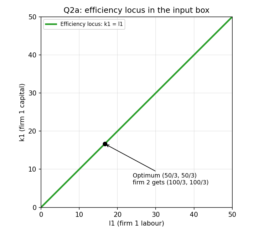
The efficiency locus is the diagonal of the input box. The dot marks the optimum found in part c.
IntuitionBoth firms have the same Cobb-Douglas exponents, so their RTS are equal exactly when both use the same capital-labour ratio. With the same totals of 50 each, that is the diagonal. Same logic as the identical-agents contract curve in Part 1. See PS_08-Production Economy, Efficiency Locus & Input Allocation.
b. Production possibility frontier (5 points)
Answer
On the locus :
c. Optimal allocation (5 points)
Answer, , ,
The slope of the PPF gives the RPT:
The consumer's MRS:
Set and use the PPF:
Inputs follow from , so and .
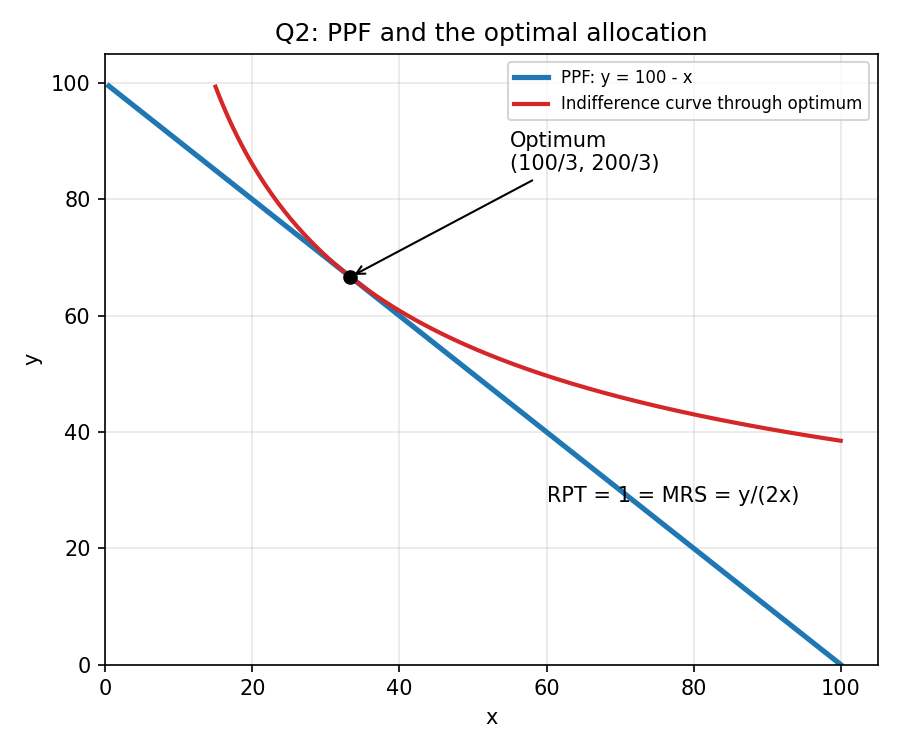
The planner picks the point where the consumer's indifference curve just touches the PPF.
d. Equilibrium prices (5 points)
Answer, , ,
Output prices. At the optimum the consumer's MRS equals the price ratio:
with as the numeraire.
Input prices. Firm 1's RTS equals the input price ratio:
Firm 1's cost function. From we get . Substituting into :
so the conditional input demands are
and is the same expression with removed. At (so ) this simplifies to
In equilibrium with :
With : , so and .
IntuitionQuick check: the firm's revenue at the optimum is , its input bill is . Zero profit, as expected for constant returns to scale.
e. Proportions with (5 points)
Answerand , i.e.
With :
so . For this reproduces part c.
IntuitionThe PPF is a straight line of slope (constant RPT), so the Cobb-Douglas consumer simply spends the expenditure share on : the output share of is .
Q3 — Partial equilibrium with a fixed price (25 points)
Demand comes from a representative consumer with quasilinear utility ( is money). Supply comes from a firm with , .
Setup used in every partFor Quasilinear Utility the inverse demand is the marginal utility, . The inverse supply is marginal cost, .
a. Cost function (5 points)
Answer
The tangency condition:
On the isoquant , so and
b. Equilibrium (5 points)
Answer,
Competitive-equilibrium benchmarks (used in part c):
| Quantity | Calculation | Value |
|---|---|---|
| Social Welfare | 1,250 | |
| Consumer Surplus | 625 | |
| Firm Surplus | 625 |
c. Government fixes the price at 60 (10 points)
AnswerQuantity . Consumer surplus 400 (down from 625), firm surplus 800 (up from 625), social welfare 1,200 (down from 1,250).
At , supply would be but demand is only . There is excess supply, so the quantity traded is the short side, demand: .
| Quantity | Calculation | Value | vs equilibrium |
|---|---|---|---|
| Social Welfare | 1,200 | falls () | |
| Consumer Surplus | 400 | falls () | |
| Firm Surplus | 800 | rises () |
Check: , so the Deadweight Loss is .
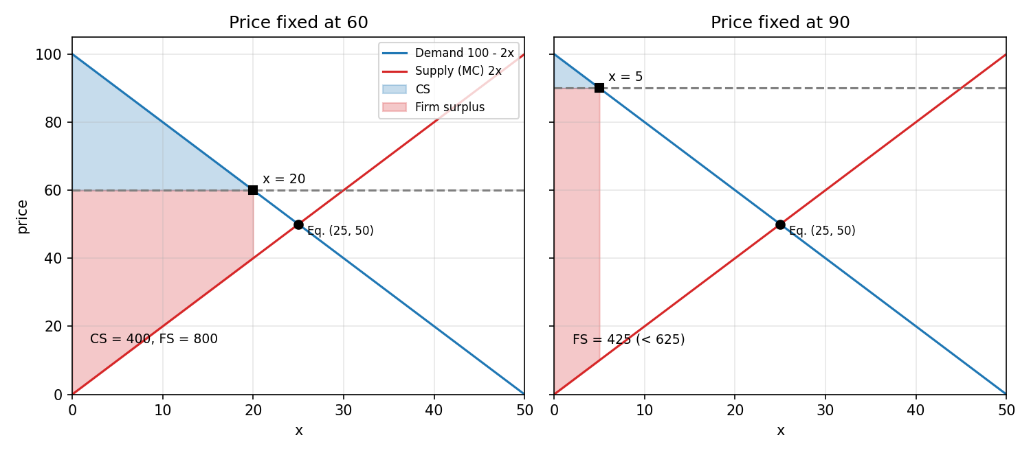
Left: a price of 60 (quantity 20). Consumers lose, firms gain. Right: a price of 90 (quantity 5), where firm surplus falls to 425.
d. Government fixes the price at 90 (5 points)
AnswerNo, the firm does not benefit: its surplus falls from 625 to 425.
At : demand gives , so (again excess supply, demand is the short side).
Economic explanation (official). The price is higher, but the quantity sold is much lower. For the producer there is a trade-off between price and quantity: the extra margin on 5 units does not make up for the surplus lost on the 20 units that are no longer sold.
Intuition: where the break-even sits (my addition, not in the official solution)For any fixed price above 50, and firm surplus is . This equals 625 at (the equilibrium) and again at , and is higher in between (for example 800 at 60). So 60 helps the firm and 90 hurts it, consistent with the official answers.
Recap table
| Part | Tool | One-line answer |
|---|---|---|
| P1 (1) | Corner solutions | False: the firm may switch corner or stay put |
| P1 (2) | Contract curve before and after | True (verdict completed from the working): old diagonal has unequal MRS once |
| P1 (3) | Rising MC with | True: optimal quantity is 0 |
| P1 (4) | Identical agents give the diagonal | True: both economies have the same contract curve |
| P1 (5) | PPF vs tastes | False: tastes pick the point, not the frontier |
| P1 (6) | Counterexample with planner | False: 10,000 vs 684 but agent 2 loses |
| P1 (7) | RTS vs | False: , only capital |
| P1 (8) | Whisky and cigars | False: marginal gain can exceed damage |
| P1 (9) | Price vs quantity effect on CS | False: lower price but lower quantity |
| P1 (10) | True: a straight line needs | |
| Q2a | Equate RTS | |
| Q2b | Substitute into | |
| Q2c | , | |
| Q2d | MRS = , | , , |
| Q2e | Same, general | , |
| Q3a | RTS = price ratio | |
| Q3b | , | |
| Q3c | Fixed price 60, short side | , , |
| Q3d | Fixed price 90 | : firm loses |
Related notes
- Micro-Economics II (hub)
- Lec_04-Theory of the Firm, Partial & General Equilibrium
- Lec_05-Production Economy & Externalities
- PS_03-Cost Minimisation & Properties of the Cost Function
- PS_04-Partial Equilibrium, Welfare & Price Ceilings
- PS_05-Pareto Efficiency, Dominance & Social Welfare
- PS_06-Exchange Equilibrium, Walrasian Prices & the Social Planner
- PS_08-Production Economy, Efficiency Locus & Input Allocation