
Quasilinear Production Economy, Exchange Equilibrium & Price Controls (2025 Moed A)
- #microeconomics
- #past-paper
- #worked-solution
- #production-economy
- #quasilinear-utility
- #corner-solution
- #partial-equilibrium
- #price-controls
- #true-false
Quasilinear Production Economy, Exchange Equilibrium & Price Controls (2025 Moed A)
Part of: Micro-Economics II Micro 2 Final Exam, Moed A (February 2025), Micro-Economics II, Dr. Boaz Zik. 3 hours, calculator only. Part 1 is 10 true/false statements (50 points); Q2 is 25 points; Q3 is 25 points. Builds on: Lec_04-Theory of the Firm, Partial & General Equilibrium, Lec_05-Production Economy & Externalities Practice: PS_02-Isoquants, RTS & Properties of the Profit Function, PS_04-Partial Equilibrium, Welfare & Price Ceilings, PS_05-Pareto Efficiency, Dominance & Social Welfare, PS_07-Core, Corner Endowments & Equilibrium vs the Social Planner, PS_08-Production Economy, Efficiency Locus & Input Allocation
SourceAnswers follow the official solutions: the 4-page Part 1 file and the 24-page open-question slides (Q2 and Q3). Where the official text has a typo or a gap, the answer is kept and a
> [!warning]callout flags it.
Question text transcribed from a scanThe question paper is an image-only scan with no text layer. All question text below was transcribed by hand from the rendered pages and cross-checked against the statements restated in the solution files. If a symbol looks odd (for example "" in statement 4, which is printed that way in the scan), the note says so.
What this paper tests
Intuition: the one move behind each part
- Part 1: every statement is a "never/necessarily" claim, so one counter-example kills it. Look for the extreme case (price near zero, a lopsided allocation).
- Q2: with a linear PPF the optimum is a corner unless the consumer's MRS happens to equal the RPT. Compare MRS with RPT.
- Q3: a fixed price sets the quantity at the short side of the market. Here both prices give , so welfare is identical and only the split of surplus changes.
Part 1 — True or false (50 points, 5 each)
The instructions say each answer needs a written argument; an answer without one scores zero.
(1) Same isoquant, shifted bundle — False
Statement. . Bundles and lie on the same isoquant. Then .
AnswerFalse. Counter-example: and .
Both bundles give , but the bundle gives , which is a lower isoquant.
IntuitionThe statement adds one unit of each input, but it mixes with . When the two bundles are far apart, is small and is small, so "adding one" to the wrong pair does not help much. The claim would be safe only for the same bundle: always beats here.
(2) Pareto dominance and a Pareto efficient allocation — False
Statement. If Pareto dominates and is Pareto efficient, then Pareto dominates .
AnswerFalse. Counter-example (utilities):
Allocation Agent 1 Agent 2 A 10 10 B 9 9 C 100 0
dominates (both agents strictly better). is Pareto efficient (agent 1 gets everything). But does not dominate : agent 2 gets .
Intuition"Pareto efficient" says nothing about being better than a particular allocation. Efficient allocations can be extremely unequal, and some of them leave one agent worse off than at . Only the efficient allocations that make everyone at least as well off as at dominate it.
(3) Change in the consumer's preferences — False
Statement. In a production economy the representative consumer's utility moves from to with . In the figure (an Edgeworth box of the two firms' inputs, with the blue efficiency locus as the diagonal), point is the optimal input allocation before the change and is the allocation after. True or false?
AnswerFalse. The figure shows a move to more and less , but the change should do the opposite.
The PPF is the same before and after, because only preferences changed, not technology. With the consumer weights more heavily (the exponent on rises from to ). The new optimum on the same PPF therefore has less and more . The figure moves along the locus in the direction of more , so it cannot be right.
IntuitionMoving along the Efficiency Locus is moving along the PPF. A taste shift towards must slide the economy towards .
(4) Equilibrium never equals the endowment — True
Statement. and , with (as printed; clearly meant ). Endowments: , . The equilibrium allocation never equals the endowment allocation.
AnswerTrue. The contract curve is the straight line for any , and the endowment is not on it.
The two agents have the same Cobb-Douglas shares (the factor 4 does not change the MRS). So gives , i.e. each agent holds the same ratio as the economy as a whole: , so . A competitive equilibrium is Pareto efficient (First Welfare Theorem), so it lies on this line. The endowment has , so it is off the line.
IntuitionAt the endowment agent 1 holds and agent 2 holds . Their MRSs differ, so there are gains from trade and the endowment cannot be an equilibrium.
(5) An allocation not Pareto dominated — False
Statement. Same preferences, , . The allocation , is not Pareto dominated by any allocation.
AnswerFalse. The contract curve is , and is not on it, so the allocation is not Pareto efficient, hence it is Pareto dominated by some allocation.
Same logic as (4): . At the ratio is . By definition, an allocation that is not Pareto efficient is dominated by some feasible allocation.
(6) A maximal price improves consumer surplus — False
Statement. In the partial equilibrium model, setting a maximal price necessarily improves consumer surplus.
AnswerFalse. Take increasing marginal cost and a ceiling close to zero.
The firm then supplies almost nothing, so quantity traded is almost zero and consumer surplus is almost zero. Without the ceiling, consumer surplus at the equilibrium price is strictly positive. So the ceiling made consumers worse off.
IntuitionA ceiling gives consumers a lower price on the units still traded but cuts the number of units. For a mild ceiling the first effect wins; for a harsh one the second does. "Necessarily" is the word that makes the statement false. See Price Ceiling.
(7) A minimal price impairs consumer surplus — True
Statement. In the partial equilibrium model, setting a minimal price necessarily impairs consumer surplus.
AnswerTrue. A minimum price forces the market price strictly above the equilibrium price, so consumer surplus is smaller than at equilibrium.
Two things hurt consumers at once: they pay more per unit, and the quantity traded falls (the short side is demand). Both effects reduce the area under the demand curve and above the price.
Reading of "minimal price"The official solution treats the floor as binding (set above the equilibrium price). A floor at or below equilibrium changes nothing, so consumer surplus would be unchanged rather than lower. State the binding assumption in your answer.
(8) Constant marginal cost and a demand increase — False
Statement. The firm's cost function is , . An increase in demand raises the firm's equilibrium profit.
AnswerFalse. Marginal cost is the constant , so in equilibrium and the firm earns zero profit whatever the demand.
Demand moves quantity, not price. Each unit sells at marginal cost, so profit per unit is zero.
IntuitionSame logic as the perfect-substitutes supply in PP_04: a flat supply curve leaves no surplus for the firm.
(9) Forced quantities and the efficiency locus — False
Statement. In an equilibrium of a production economy, firm 1 (2) is required to produce () different from the equilibrium quantity (). The demanded quantities of labour and capital necessarily correspond to a point on the efficiency locus.
AnswerFalse. As in the class proof that the equilibrium allocation is optimal, equilibrium prices only clear the input markets at the equilibrium quantities.
At other forced quantities, the firms' cost-minimising demands at those prices need not add up to the available inputs: one input is over-demanded and the other under-demanded. Inputs would not be fully allocated, so the point is not on the Efficiency Locus.
(10) MRS above RPT — False
Statement. On the PPF at a point where the consumer's MRS is strictly greater than the RPT, the amount of is greater than under the optimal allocation.
AnswerFalse. The amount of at that point is smaller than at the optimum.
If , the consumer values an extra unit of (in terms of ) more than the economy has to give up to produce it. The economy should move along the PPF towards more and less , so the optimal is greater than at this point.
Q2 — Production economy with quasilinear utility (25 points)
Setup. Two firms: and , . The representative consumer has . Resources: and . Firm 1 makes , firm 2 makes .
A stray "b" in the official slidesThe printed question has no in , but the official slides carry a factor in and in the corner answer . The slide that gives the PPF drops it (), and the later answers (, ) also use . This note follows the printed question, so . See the "Economic reasoning" box in part 2 for the role plays when it is present.
1a — Efficiency locus (3 points)
Answer(the diagonal of the input box).
Efficiency needs (see Efficiency Locus), so . Cross-multiplying: , so , i.e. .
1b — Production possibility frontier (3 points)
Answer
On the locus , so . Firm 2 gets the rest, , so .
IntuitionBoth firms are constant returns to scale and have the same technology, so at equal input ratios one unit of "input pair" makes one unit of either good. The RPT is therefore at every point: the PPF is a straight line.
1c — Optimal allocation with (4 points)
Answer, , , .
With the at every point, while the everywhere. Since (the consumer would pay 2 units of for a unit of but only has to give up 1), the economy should keep shifting resources to until it runs out: a corner solution. All inputs go to firm 1.
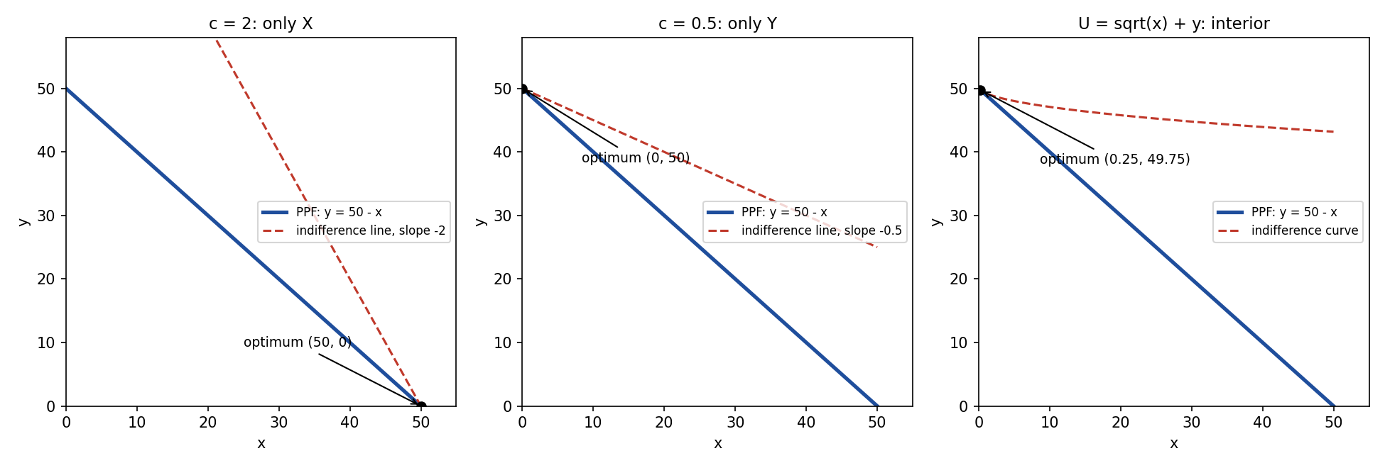
Left panel: the indifference line (slope ) is steeper than the PPF (slope ), so utility is highest at the corner.
2 — Optimum with , and why it differs (5 points)
Answer, (the official slides write ), with and .
Now : giving up a unit of to make a unit of costs more (1) than the consumer will pay (0.5). So only is produced. The corner flips from (part 1c) to (middle panel above).
Official economic reasoningThe optimum is a corner: only or only is produced. Two things decide which:
- the relative productivity of , shown by : how many units of the economy gets for giving up one unit of (the slope of the PPF);
- the relative utility of , shown by : how many units of the consumer would pay for one unit of .
If is above the PPF slope, produce only ; if below, produce only .
IntuitionWith a linear PPF and linear utility, there is no curvature to balance the two goods. The comparison is "my willingness to pay" against "the economy's opportunity cost", and the larger one wins everything.
3 — Optimum with (5 points)
Answer, .
The PPF is unchanged (, ), but the MRS now depends on , so an interior solution exists. Set :
Then (right panel above).
4 — Doubling the resources (5 points)
Answerstays at ; rises to .
Doubling both inputs (, ) shifts the PPF out to . The RPT is still , and the MRS still equals , which depends only on . So gives again, and .
Official economic reasoningBecause utility is quasilinear, the demand for does not depend on income or resources (no income effect). All the extra resources go to .
See Quasilinear Utility for why the good that enters linearly absorbs all changes in wealth.
Q3 — Partial equilibrium with fixed prices (25 points)
Setup. Two goods: and (money). Consumer utility (income high enough that there are no corner solutions). Supply by a representative firm with , input prices .
(a) Cost function (8 points)
Answer, with supply .
Cost minimisation: , so . Then , so . Therefore
(b) Competitive equilibrium (7 points)
Answer, .
Demand is the marginal utility: (see Quasilinear Utility). Setting gives , so and .
Surpluses at the competitive equilibrium (used in (c))
(c) Government fixes (5 points)
Answer, , , . Changes: , , .
A price of 90 is above the equilibrium price (a floor). At 90, demand is , while the firm would supply . The short side is demand, so trade is .
Against the competitive equilibrium: , , .
Official wordingThe slide says "there would be excess demand" at 90. In fact at there is excess supply ( supplied versus demanded). The number is correct and is what the calculation uses.
(d) Government fixes (5 points)
Answer, , , .
A price of 60 is below equilibrium (a ceiling). At 60, the firm supplies , while demand is . The short side is supply, so trade is again .
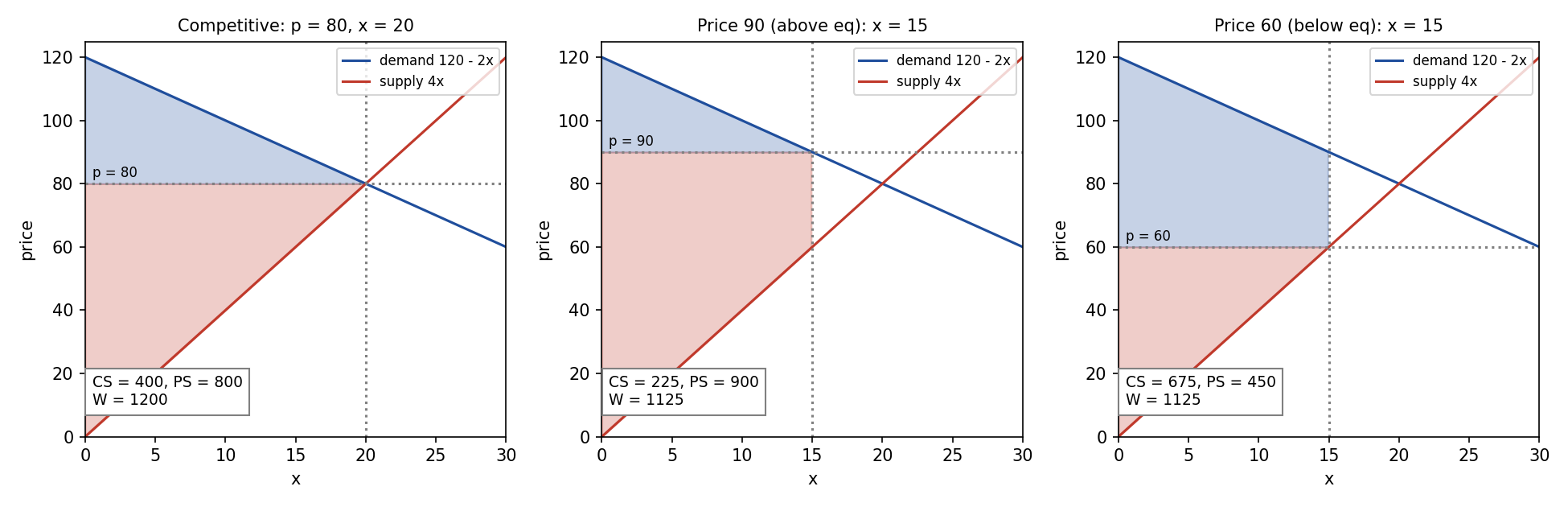
Same quantity (15) at both prices. At 90 the firm collects the rent between demand and supply; at 60 the consumers do.
Official comparison of (c) and (d)At both prices the quantity traded is . The difference is who gets the "green" surplus on the traded units: the firm when , the consumers when . Total welfare is the same () because the quantity is the same; both prices lose against the competitive , the Deadweight Loss from the units between and that are not traded.
Assumption behind the numbersThe consumer surplus integral assumes that the 15 units go to the consumers who value them most (efficient rationing). If the units were allocated differently, at would be lower. The official solution makes this assumption without saying so.
Recap table
| Part | Tool | One-line answer |
|---|---|---|
| P1 (1) | Counter-example on | False: give , but gives |
| P1 (2) | Utility table | False: efficient but not above |
| P1 (3) | Same PPF, taste shift | False: means more , less |
| P1 (4) | Contract curve | True: endowment is off the line |
| P1 (5) | Contract curve | False: is inefficient, so dominated |
| P1 (6) | Ceiling near zero | False: quantity and go to about |
| P1 (7) | Binding floor | True: higher price, lower quantity |
| P1 (8) | Constant MC | False: , profit is |
| P1 (9) | Prices clear only at equilibrium quantities | False: inputs not fully allocated |
| P1 (10) | False: optimum has more | |
| Q2-1a | ||
| Q2-1b | Substitute the locus | |
| Q2-1c | , | |
| Q2-2 | , | |
| Q2-3 | , | |
| Q2-4 | Quasilinear: no income effect | , |
| Q3a | RTS = price ratio | , |
| Q3b | , | |
| Q3c | Short side at | , , |
| Q3d | Short side at | , , |
Related notes
- Micro-Economics II (hub)
- Lec_04-Theory of the Firm, Partial & General Equilibrium
- Lec_05-Production Economy & Externalities
- PS_02-Isoquants, RTS & Properties of the Profit Function
- PS_04-Partial Equilibrium, Welfare & Price Ceilings
- PS_05-Pareto Efficiency, Dominance & Social Welfare
- PS_07-Core, Corner Endowments & Equilibrium vs the Social Planner
- PS_08-Production Economy, Efficiency Locus & Input Allocation