
Production Economy, Price Floor & Ceiling, Exchange True-False (2023 Moed B)
- #microeconomics
- #past-paper
- #worked-solution
- #true-false
- #production-economy
- #efficiency-locus
- #ppf
- #social-planner
- #partial-equilibrium
- #price-floor
- #price-ceiling
Production Economy, Price Floor & Ceiling, Exchange True-False (2023 Moed B)
Part of: Micro-Economics II Micro 2 Final Exam, Moed Bet (March 2023), Micro-Economics II, Dr. Boaz Zik. 3 hours, cheat sheet and calculator allowed. Part 1 is 50 points (ten true/false items, 5 points each); Q2 and Q3 are open questions. Builds on: Lec_04-Theory of the Firm, Partial & General Equilibrium, Lec_05-Production Economy & Externalities Practice: PS_04-Partial Equilibrium, Welfare & Price Ceilings, PS_05-Pareto Efficiency, Dominance & Social Welfare, PS_06-Exchange Equilibrium, Walrasian Prices & the Social Planner, PS_07-Core, Corner Endowments & Equilibrium vs the Social Planner, PS_08-Production Economy, Efficiency Locus & Input Allocation
SourceThe paper has two official solution files. Part 1 has only the circled True/False verdicts (no reasoning), so every explanation below is written here, not copied. Q2 and Q3 follow the worked official solution (the 7th page of that file is blank). All ten verdicts and every number were re-checked and agree with the official ones. Where the official text has a typo it is flagged with a
> [!warning].
What this paper tests
Intuition: the one move behind each open question
- Q2: efficient production means equal RTS across firms, which gives the efficiency locus; the PPF then turns inputs into outputs, and the optimum is where the consumer's MRS equals the RPT (the PPF slope).
- Q3: demand is the marginal utility, supply is marginal cost. A price fixed by the government means the short side of the market trades: demand if the price is above equilibrium, supply if it is below.
Part 1 — True or false (50 points)
Answer key
| # | Statement in short | Official verdict |
|---|---|---|
| 1 | Swapping the Cobb-Douglas exponents between the agents leaves the contract curve unchanged | False |
| 2 | Economy 2 equilibrium gives each agent twice the of economy 1 | True |
| 3 | A higher in the consumer's utility shifts the PPF out in | False |
| 4 | Planner prefers to , and Pareto dominates , so planner prefers to | True |
| 5 | and are always on the contract curve | True |
| 6 | Quasilinear technology: marginal cost equals beyond some quantity | True |
| 7 | A consumer price subsidy lowers social welfare | True |
| 8 | The planner always prefers equilibrium to any allocation off the contract curve | False |
| 9 | Non-equilibrium positive prices give excess demand for one good and excess supply of the other | True |
| 10 | Equilibrium utility is at least endowment utility | True |
1. Same contract curve after swapping exponents? (False)
AnswerFalse. Swapping which agent has exponent and which has changes the contract curve unless .
Write and , with because . The Contract Curve is where , with :
Economy 1 (agent 1 has , agent 2 has ):
Economy 2 swaps the roles ( and exchange places):
At the box centre economy 1 gives and economy 2 gives . These differ whenever , so the curves differ.
IntuitionThe curve bows towards the agent who likes more. In economy 1 that is agent 1 (who has the smaller exponent on ); in economy 2 it is agent 2. The curves are mirror images of each other, not the same curve.
2. Twice the in economy 2? (True)
AnswerTrue.
In each economy the two agents are identical (same Cobb-Douglas exponent) and have the same endowment. Then the equilibrium is the no-trade allocation: each agent consumes their own endowment. Both want the same bundle at any price ratio, so the market clears with each keeping what they have.
- Economy 1: each agent consumes , so .
- Economy 2: each agent consumes , so .
.
IntuitionThe exponents and are a distraction. When both agents are clones with identical endowments, there are no gains from trade, so the equilibrium allocation equals the endowment.
3. Does a change in preferences move the PPF? (False)
AnswerFalse. The PPF is built from the firms' technologies and the resource constraints only. Preferences do not enter it.
A move from to puts more weight on , which moves the optimal point along the PPF towards more (the MRS curve changes), but the frontier itself stays where it is.
4. Transitivity with Pareto dominance (True)
AnswerTrue.
Two facts about the planner: (i) the planner's preferences are transitive; (ii) the planner respects Pareto dominance, because social welfare is increasing in each agent's utility, so if dominates the planner prefers to . Then and give .
AssumptionThis needs a planner whose welfare is increasing in the agents' utilities (as in the course's Cobb-Douglas planner of PS_05-Pareto Efficiency, Dominance & Social Welfare). A planner who ignored Pareto dominance could break the chain.
5. Are the origins always on the contract curve? (True)
AnswerTrue.
At agent 2 holds the entire endowment of both goods. Any move gives agent 1 something and so must take it from agent 2, who strictly prefers more of each good (Local Nonsatiation). So no Pareto improvement exists: the allocation is Pareto efficient. The same holds for .
IntuitionThe contract curve in the Edgeworth box runs corner to corner, from to . Efficiency says nothing about fairness, so "one agent gets everything" is efficient.
6. Quasilinear technology and marginal cost (True)
AnswerTrue.
With and concave, (decreasing) and . The RTS is , and the Tangency Condition is , which fixes labour at one constant level regardless of output.
- For small (below ) the firm hits the corner and uses only labour.
- For labour stays at and all extra output comes from capital: .
So for large :
Beyond the threshold , marginal cost equals the price of capital.
7. Consumer price subsidy in partial equilibrium (True)
AnswerTrue (social welfare falls).
A subsidy to buyers pushes trade above the competitive quantity. For the extra units, the marginal cost exceeds the marginal value, so each extra unit destroys value. Counting the government's cost of the subsidy, social welfare falls by the Deadweight Loss triangle. Only at the competitive quantity is maximised.
8. Planner prefers equilibrium to any off-curve allocation? (False)
AnswerFalse.
A planner who puts heavy weight on one agent can prefer an allocation that gives that agent much more, even if that allocation is inefficient, to a balanced equilibrium. Being off the contract curve only means some allocation Pareto dominates it, not that the equilibrium beats it for this planner.
What would make it trueThe statement would be true for any allocation that the equilibrium Pareto dominates, since a planner who respects Pareto dominance prefers the equilibrium to those. It is not true for every off-curve allocation.
9. Prices that are not an equilibrium (True)
AnswerTrue.
Walras' Law: for any positive prices, where is excess demand. If then forces , which would be an equilibrium. So at non-equilibrium prices both and are non-zero, and since with positive prices they have opposite signs: excess demand for one good and excess supply of the other.
10. Equilibrium utility vs endowment utility (True)
AnswerTrue.
The endowment is always affordable (it costs exactly the agent's income), so the agent could choose it. The optimum on the same budget set is at least as good: . This is Individual Rationality; it is why every equilibrium lies in the Core-style "lens" inside the box.
Q2 — Production economy (points not stated in the sources)
Firms: and . Representative consumer . Resources: and .
Typo in the question paperThe printed utility reads . The solution uses , so the "" is a typo for .
a. Efficiency locus
Answer
Efficient production needs (Efficiency Locus). For firm 1:
Firm 2 is identical, so . Equating:
Cross-multiplying: , so , i.e. .
Minor typo in the official workingThe official text prints the marginal products without the constant 2 from the production function ( and ). The factor 2 multiplies both and cancels in the ratio, so and the answer are unaffected.
IntuitionBoth firms have the same technology, so efficiency means they use inputs in the same proportion. In the input box that is the diagonal.
b. Production possibility frontier
Answer
On the locus and :
So and .
c. Optimal allocation
Answer, , , .
The RPT is the (absolute) slope of the PPF, which is . The consumer's MRS:
Set : , so . Into the PPF: , so and . Then and , with in each firm.
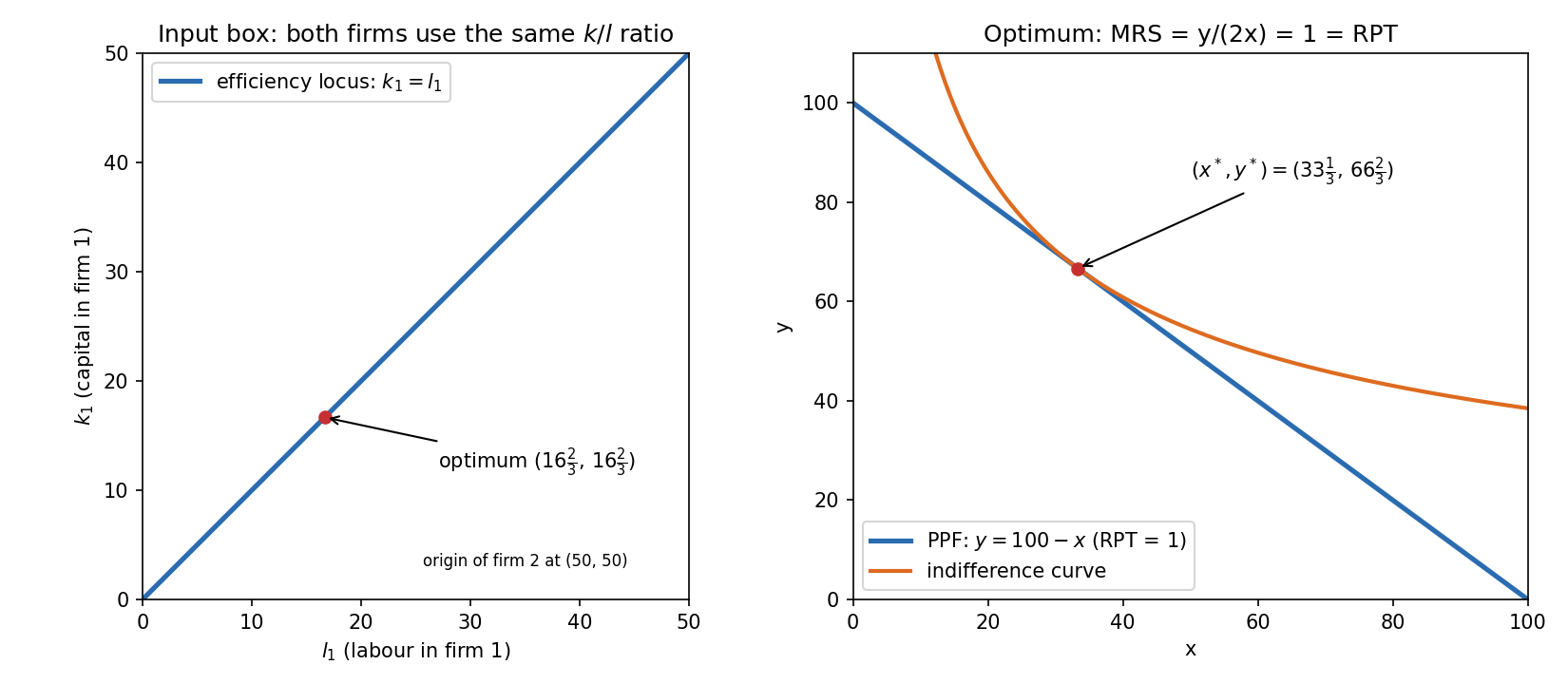
Left: the efficiency locus is the diagonal of the input box and the optimum sits on it. Right: the optimum is where the indifference curve is tangent to the PPF.
d. Equilibrium prices
Answer(with as numeraire), , .
At the optimum . With :
Firms: cost minimisation requires . At this is , so and as expected. Firm 1's cost to produce (so ):
Profit maximisation gives , so :
Check (not in the official solution)Firm 1 revenue , cost , so profit is zero, as constant returns require. Total input income .
e. Technology change:
Answerstays the same, increases, so the ratio increases. Good is now relatively cheaper to produce.
The efficiency locus is still (the constant 4 cancels in the RTS). With :
The new PPF has . With we get , so and , . The ratio rises from to .
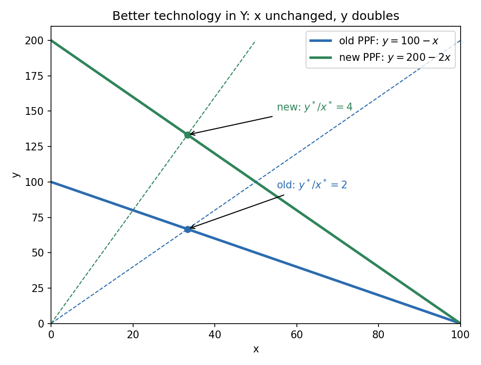
The PPF pivots out around its -intercept (100, 0), because only the -technology improved. The optimum moves up along the ray (steeper than the old ray ).
IntuitionThe official answer is graphical: production is relatively better, and with Cobb-Douglas preferences the consumer's choice of does not change, while rises. The algebra above confirms it: before and after, goes from to .
Q3 — Partial equilibrium, a price above and a price below equilibrium
Demand from a consumer with ( is money, income high enough for an interior solution). Supply from a firm with and .
a. Cost function
Answer
The tangency condition is , so . The isoquant is , so , and
Marginal cost, which is the supply curve, is .
b. Equilibrium
Answer,
For Quasilinear Utility the inverse demand is the marginal utility of : . The inverse supply is . Equate: , so and .
At equilibrium (reference level for parts c and d):
c. Government price of 90
AnswerQuantity traded . (down 175), (up 100), (down 75).
Price is above the equilibrium price of 80. At 90 buyers want , so units, while firms would supply , i.e. units. Supply exceeds demand, so the short side, demand, sets the quantity: .
| Equilibrium (80) | Price 90 | Change | |
|---|---|---|---|
| Consumer surplus | 400 | 225 | |
| Firm surplus | 800 | 900 | |
| Social welfare | 1200 | 1125 |
Firms gain because they sell fewer units but at a much higher price; consumers lose on both price and quantity; the net loss of 75 is the Deadweight Loss.
Mislabelled in the official textThe official solution calls the situation at 90 "excess demand". At a price above equilibrium there is excess supply (22.5 supplied vs 15 demanded). The number is correct. It also writes "the supply in the market would be ", meaning the quantity traded is read off the demand curve.
d. Government price of 60
AnswerQuantity traded . , , .
Price is below equilibrium. At 60 buyers want , i.e. units, but firms supply only , i.e. units. Now supply is the short side and .
| Price 90 | Price 60 | |
|---|---|---|
| Quantity traded | 15 | 15 |
| Consumer surplus | 225 | 675 |
| Firm surplus | 900 | 450 |
| Social welfare | 1125 | 1125 |
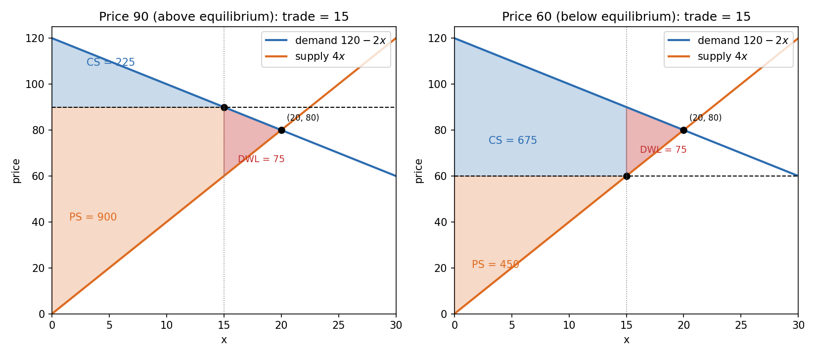
Both prices cut trade to 15 units, so both lose the same deadweight triangle between 15 and 20 (area 75). Only the split between consumers and the firm differs.
Explanation (comparison with part c)Social welfare is the same (1125) because welfare depends only on the quantity traded, and the quantity is 15 in both cases. The price only decides who gets the surplus. At 90 the firm captures more of the pie; at 60 consumers do. The gap between equilibrium welfare (1200) and 1125 is the deadweight loss of 75 in both.
Assumption in the consumer surplusComputing as assumes the 15 units go to the buyers who value them most (efficient rationing). With a price at 60 and demand for 30 units, a different rationing rule would give a lower .
Recap table
| Item | Tool | Answer |
|---|---|---|
| P1 (1) | Contract curve from MRS equality, swap and | False |
| P1 (2) | Identical agents and endowments: no trade | True |
| P1 (3) | PPF is technology only | False |
| P1 (4) | Transitivity plus Pareto-respecting planner | True |
| P1 (5) | Origins are efficient (one agent holds everything) | True |
| P1 (6) | Quasilinear technology: capital is the marginal input | True |
| P1 (7) | Subsidy pushes quantity above efficient | True |
| P1 (8) | Planner weights can favour an inefficient allocation | False |
| P1 (9) | Walras' Law with non-equilibrium prices | True |
| P1 (10) | Endowment is affordable | True |
| Q2a | RTS equality | |
| Q2b | Substitute locus into production | |
| Q2c | ||
| Q2d | Cost function and | , |
| Q2e | New PPF | same, up, ratio 2 to 4 |
| Q3a | Tangency | |
| Q3b | Demand = supply | |
| Q3c | Price 90, demand is short side | , , |
| Q3d | Price 60, supply is short side | , , |
Related notes
- Micro-Economics II
- Lec_04-Theory of the Firm, Partial & General Equilibrium, Lec_05-Production Economy & Externalities
- PS_04-Partial Equilibrium, Welfare & Price Ceilings, PS_05-Pareto Efficiency, Dominance & Social Welfare, PS_06-Exchange Equilibrium, Walrasian Prices & the Social Planner, PS_07-Core, Corner Endowments & Equilibrium vs the Social Planner, PS_08-Production Economy, Efficiency Locus & Input Allocation