
Production Economy, Price Ceiling & True-False (2025 Moed B)
- #microeconomics
- #past-paper
- #worked-solution
- #true-false
- #production-economy
- #price-ceiling
- #partial-equilibrium
- #social-welfare
Production Economy, Price Ceiling & True-False (2025 Moed B)
Part of: Micro-Economics II Micro 2 Final Exam, Moed B (March 2025), Micro-Economics II, Dr. Boaz Zik. 3 hours, calculator only. Part 1 (10 true/false, 5 points each = 50 points), Question 2 (25 points), Question 3 (25 points). Builds on: Lec_04-Theory of the Firm, Partial & General Equilibrium, Lec_05-Production Economy & Externalities Practice: PS_01-Profit Maximisation & Properties of the Profit Function, PS_03-Cost Minimisation & Properties of the Cost Function, PS_04-Partial Equilibrium, Welfare & Price Ceilings, PS_05-Pareto Efficiency, Dominance & Social Welfare, PS_06-Exchange Equilibrium, Walrasian Prices & the Social Planner, PS_08-Production Economy, Efficiency Locus & Input Allocation
SourceThe question paper is an image-only scan, so the question text below was transcribed from the scan by eye (a few handwritten marks on the scan are ignored). Part 1 and Q3 follow the official solutions. Question 2 has no official solution anywhere, so its text is transcribed and every part is marked as unsolved.
Question 2 is unsolvedNo official solution exists for Q2 in the course materials. It is deliberately not solved here. See PS_08-Production Economy, Efficiency Locus & Input Allocation and Lec_05-Production Economy & Externalities for the method.
What this paper tests
Intuition: the one move behind each block
- Part 1: for each statement ask "what is the object, and what does it depend on?" (a price ratio, a homogeneous function, an aggregate endowment).
- Q3: with a binding maximal price the short side decides quantity. Supply is the short side, so quantity solves , and the demand curve only enters through consumer surplus.
Part 1 — True or false (50 points)
For each statement, state if it is true or false and provide a written argument for your answer (an answer without an argument will be marked zero).
(1) Cost after a rise in (5 points)
Question. Consider a firm with production function . Suppose the price of , , increases while remains constant. Following this change, the cost of producing any quantity strictly increases. True/False.
Answer: FalseFor small enough quantities the firm would choose to produce only with labour, both before and after the change in . For these quantities the cost of production remains the same.
Why. The statement says "any quantity", so one counterexample is enough. A rise in can only hurt through the capital the firm uses. If the firm uses no capital at , the rise changes nothing.
Intuition (mine, consistent with the official argument)The marginal product of labour, , is huge when is small, while the marginal product of capital is constant at 1. So at small labour is the better buy per dollar even at the old , and the firm is at the labour corner (Corner Solution). Raising makes capital even less attractive. At large the firm does use capital and cost does rise, which is why the statement fails only because of the word "any".
(2) Wage and product price rise together (5 points)
Question. A firm produces using only labour, with diminishing marginal productivity: with strictly concave. If both the wage and the product price increase by the same proportion, then the firm's optimal profit remains unchanged. True/False.
Answer: FalseThe firm's optimal profit increases in the same proportion as and .
Why. The firm solves . Scaling by scales the whole objective by , so the optimal is unchanged but the profit is times larger. This is Homogeneity of Degree 1 of the Optimal Profit Function: . Only relative prices change the firm's decision; the level of profit scales with them.
(3) Both input prices rise together (5 points)
Question. A firm has . If both and increase by the same proportion, then the firm's optimal input bundle for producing a given quantity remains unchanged. True/False.
Answer: TrueThe cost-minimising bundle for depends only on the input price ratio , and this ratio does not change when both prices rise by the same proportion.
Why. The tangency condition Tangency Condition is , and with Cobb-Douglas . Together with this pins down using the ratio alone. The cost rises by the same proportion, but the bundle does not. See Cost Minimisation and Conditional Input Demand.
(4) Subsidy financed by a lump-sum tax (5 points)
Question. In a partial equilibrium model the government subsidises the price for consumers. To finance the subsidy, the government imposes a direct (lump-sum) tax on consumers. As a result, consumer surplus decreases compared to the scenario with no intervention. True/False.
Answer: TrueIf we ignore the financing, both consumer surplus and firm surplus increase. When we account for financing, overall welfare decreases. Since the consumers pay for the subsidy, consumer surplus decreases.
Why. The subsidy pushes the quantity above the efficient level, creating a Deadweight Loss. The firm gains from the subsidy and the consumer gains from the lower price, but the consumer also pays the entire bill through the lump-sum tax. Total welfare is the sum of the surpluses (the tax is a transfer from consumers to the government that is paid back to firms and consumers through the subsidy). Welfare falls by the deadweight loss, and the firm is better off, so the consumer must be worse off than with no intervention.
Intuition (mine)The consumer is paying the firm to sell extra units that the consumer values at less than they cost to produce. The firm is happy to be paid; the consumer carries both the transfer and the waste.
(5) Minimum price equal to the subsidised price (5 points)
Question. The government does not implement a subsidy but instead sets a minimum price equal to the price under the subsidy policy of (4). Under this policy, the firm's surplus remains the same as it was following the subsidy policy in (4). True/False.
Answer: FalseWhen the minimum price equals the subsidy price (and is above the equilibrium price), consumers demand less. The firm therefore sells a smaller quantity at the same price per unit, so its profit decreases relative to the subsidy policy of (4).
Why. Under a minimum price above equilibrium, the market is on the demand curve (the short side), so quantity is whatever consumers want at that price. Under the subsidy the quantity is larger (consumers face a lower effective price). Same unit price, fewer units sold, and units beyond the new quantity carried positive firm surplus, so the firm's surplus falls.
(6) Endowment on the contract curve (5 points)
Question. In an exchange economy where the initial endowment allocation lies on the contract curve, agents do not benefit from trade. True/False.
Answer: TrueIf the endowment is on the contract curve, the equilibrium allocation equals the endowment. Agents therefore do not benefit from trade.
Why. On the Contract Curve the allocation is already Pareto efficient, so no trade can make someone better off without hurting the other. The Walrasian equilibrium is individually rational and efficient, so it must be the endowment itself. See Walrasian Equilibrium and Core.
(7) A higher equilibrium (5 points)
Question. In an exchange economy a change raises the equilibrium price relative to its previous level. In the new equilibrium, both agents consume less of good . True/False.
Answer: FalseIn an exchange-economy equilibrium the agents consume the overall endowment. So total consumption of is the same under any equilibrium. It is impossible for both agents to consume less.
Why. Market clearing gives , a fixed number. A price change can shift from one agent to the other, but cannot lower both. A rise in can at most move between the two agents.
(8) Doubling the input endowments (5 points)
Question. In a production economy the representative consumer has . The firms have and , with and . The input endowments change to and . In the new equilibrium, the quantities of both and are twice their previous equilibrium levels. True/False.
Answer: TrueIf and , the optimal consumption of and is proportional to . It is the same as the Cobb-Douglas consumer problem with price ratio 1 and income . Since the resource constraints doubled, so do the optimal quantities.
Why. Both firms are constant-returns Cobb-Douglas with the same technology, so the PPF is the line when and both equal (the official solution treats the price ratio as 1). The consumer then spends the share of income on and on : and . Doubling doubles both. See Production Economy and PS_08-Production Economy, Efficiency Locus & Input Allocation.
(9) A point on the PPF and equal RTS (5 points)
Question. In a production economy, assume lies on the production possibility frontier. There exist two points on the isoquant of and on the isoquant of , such that . True/False.
Answer: TrueIf is on the PPF there is an allocation of inputs along the efficiency locus that produces this output. That allocation has on the isoquant of and on the isoquant of , and satisfies .
Why. The PPF is built from the Efficiency Locus, where the two firms' isoquants are tangent (equal RTS). A point is on the PPF only if it is produced efficiently, which means equal RTS across firms.
(10) A non-Pareto-efficient allocation and the planner (5 points)
Question. If allocation is not Pareto efficient, then no central benevolent designer would select it. True/False.
Answer: TrueA benevolent designer's utility must increase in the utilities of the agents. Since is not Pareto efficient, there is another allocation giving higher utility to all agents. Any benevolent designer prefers to , so no such designer would select .
Why. A planner's objective is increasing in each agent's utility (Social Welfare). A Pareto-dominating allocation raises every argument, so it raises the objective. See PS_05-Pareto Efficiency, Dominance & Social Welfare.
Q2 — Production economy (25 points)
No official solutionThe question is transcribed from the scan. There is no official solution for Q2 in any of the course files, so no part is solved here.
Question. Consider the following production economy. The firms' production functions are and . The representative consumer's utility function is and the resource constraints are and .
a. Efficiency locus (5 points)
Find the efficiency locus in the economy.
No official solution
b. Production possibility frontier (5 points)
Find the production possibility frontier.
No official solution
c. Optimal allocation (5 points)
Find the optimal allocation in the economy.
No official solution
d. Equilibrium prices (5 points)
Find the equilibrium prices.
No official solution
e. Change in firm 2's technology (5 points)
Assume now that and . What will happen to the ratio in the optimal allocation of and ? Explain your answer via graphical illustration.
No official solution
Q3 — Partial equilibrium with a maximal price (25 points)
Setup. A market with two products and , where represents money. Demand comes from a representative consumer with utility
(income is high enough that there are no corner solutions). Supply is set by a representative firm with production function
and input prices and .
a. Numerical case: and
(i) The firm's cost function (4 points)
Answer
Cost minimisation (Cost Minimisation): set . For this production function , and with equal prices this equals 1, so . Put this in the isoquant , so
(ii) Equilibrium price, quantity and surpluses (4 points)
Answer, , consumer surplus , firm surplus , social welfare .
The consumer maximises subject to income. Quasilinearity gives inverse demand (Quasilinear Utility). Marginal cost is . Equilibrium solves
The surpluses are
and Social Welfare is . See Consumer Surplus and Firm Surplus.
(iii) A maximal price of 80 (4 points)
AnswerQuantity , consumer surplus , firm surplus , social welfare .
Equilibrium Maximal price 80 Change Quantity 30 20 falls Consumer surplus 900 1600 rises Firm surplus 1800 800 falls Social welfare 2700 2400 falls
The maximal price 80 is below the equilibrium price 120, so it binds. At price 80 consumers want more than firms will supply, so supply is the short side and quantity solves :
Social welfare is , a Deadweight Loss of relative to .
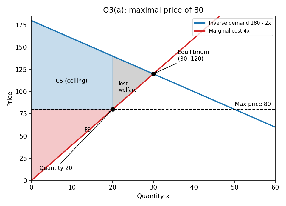
The maximal price caps the quantity at 20 where marginal cost meets the price cap. The grey triangle is the welfare lost relative to the equilibrium.
Explanation (official). Consumer surplus increases: the lower price more than compensates the consumer for the lower quantity. Firm surplus decreases: the firm sells fewer units and at a lower price. Social welfare decreases because the allocation no longer coincides with the equilibrium allocation.
Typos in the official solutionThe official text says "The consumer surplus equal " and later "The consumer surplus decreased". Both slips should read firm surplus. The numbers (1600 and 800) are right: and .
IntuitionWelfare drops because some trades worth doing (units between 20 and 30, where willingness to pay exceeds marginal cost) no longer happen. The consumer wins on the units that do trade (price 80 instead of 120), the firm loses on them.
b. Demand rises under a binding maximal price (5 points)
Question. Consider the general market (not the numbers of (a)). The government sets a maximal price smaller than the equilibrium price. Now there is an increase in demand, captured by an increase in the parameter (same maximal price). What happens to firm surplus and consumer surplus compared with before the change? Give verbal and graphical explanations.
AnswerFirm surplus is unchanged. Consumer surplus increases.
An increase in shifts demand up, so the equilibrium price rises and the maximal price is still below it. The quantity is therefore still set where marginal cost equals the maximal price. Marginal cost does not depend on , so the quantity is unchanged. The firm sells the same quantity at the same price with the same cost, so
does not change. Consumer surplus is
and even though and do not change, rises, so rises.
c. Input prices fall under a binding maximal price (5 points)
Question. Same setup, but now the input prices and decrease (same maximal price). What happens to firm surplus and consumer surplus?
AnswerBoth consumer surplus and firm surplus increase.
A fall in input prices lowers marginal cost. Quantity is set where price equals marginal cost, so the quantity rises. The price stays equal to the maximal price. Consumer surplus rises because it increases in the quantity at a given price. Firm surplus also rises because marginal cost fell, so the firm earns more on every unit sold.
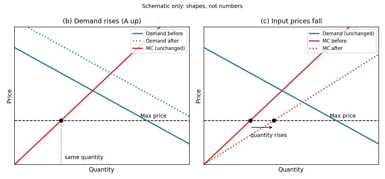
Left: a demand shift (b) leaves the quantity at the unchanged supply point. Right: a fall in costs (c) moves that point to the right. Schematic, no numbers.
d. Why (b) and (c) differ (3 points)
AnswerIn (b) a demand increase leaves the quantity unchanged because, under a binding maximal price, the quantity is set by supply, which did not change. Only the consumer benefits. In (c) a cost decrease raises the supply, so the quantity changes, and both the firm and the consumer benefit.
IntuitionA price cap makes the market supply-determined. Anything that shifts only demand is invisible to the firm and benefits consumers through the surplus formula. Anything that shifts supply changes the quantity actually traded, so it matters to both sides.
Recap
| Item | Verdict or answer | One-line reason |
|---|---|---|
| (1) | False | Small : labour only, so cost does not change |
| (2) | False | Profit is homogeneous of degree 1, scales with the prices |
| (3) | True | Bundle depends only on |
| (4) | True | Consumer bears the lump-sum tax and the deadweight loss |
| (5) | False | A minimum price cuts quantity, firm sells less |
| (6) | True | Endowment on contract curve means no trade |
| (7) | False | Total fixed, one agent can only gain what the other loses |
| (8) | True | Doubling doubles and (Cobb-Douglas, price ratio 1) |
| (9) | True | PPF points are produced on the efficiency locus (equal RTS) |
| (10) | True | A Pareto-dominating allocation raises any planner's objective |
| Q2 | No official solution | Not solved |
| Q3(a)(i) | ||
| Q3(a)(ii) | , , , , | |
| Q3(a)(iii) | , , , | |
| Q3(b) | same, up | Quantity set by unchanged supply |
| Q3(c) | up, up | Lower raises quantity |
| Q3(d) | Different | Only supply shifts move the quantity under a cap |