
True-False Mix, Production Economy & Subsidy vs Price Cap (2023 Moed A)
- #microeconomics
- #past-paper
- #worked-solution
- #true-false
- #production-economy
- #efficiency-locus
- #ppf
- #subsidy
- #price-ceiling
True-False Mix, Production Economy & Subsidy vs Price Cap (2023 Moed A)
Part of: Micro-Economics II Micro 2 Final Exam, Moed A (20/02/2023), Micro-Economics II, Dr. Boaz Zik. 3 hours, cheat sheet and calculator allowed. Part 1: ten true/false statements (5 points each, 50 total). Part 2: two open questions (Q2 = 25 points, Q3 = 25 points). Builds on: Lec_04-Theory of the Firm, Partial & General Equilibrium, Lec_05-Production Economy & Externalities Practice: PS_01-Profit Maximisation & Properties of the Profit Function, PS_02-Isoquants, RTS & Properties of the Profit Function, PS_03-Cost Minimisation & Properties of the Cost Function, PS_04-Partial Equilibrium, Welfare & Price Ceilings, PS_05-Pareto Efficiency, Dominance & Social Welfare, PS_06-Exchange Equilibrium, Walrasian Prices & the Social Planner, PS_08-Production Economy, Efficiency Locus & Input Allocation
SourceAnswers follow the official solutions. The true/false key is a 2-page PDF that repeats the statements with the correct word underlined (no explanations), so the reasons below are written for revision, not copied. The open-question solution is 6 pages. Where the official text has a typo or a gap, the answer is kept and a
> [!warning]flags it.
What this paper tests
Intuition: the one move behind each part
- True/false: for each statement ask "what is held fixed, and what does the statement quietly assume?". Most false statements fail on a hidden "for any" or "at every level".
- Q2: equalise the two firms' RTS to get the efficiency locus, plug into the outputs to get the PPF, then set RPT equal to the consumer's MRS.
- Q3: price equals marginal cost on the supply side, price equals marginal utility on the demand side. A subsidy shifts a curve; a price cap makes the short side of the market decide the quantity.
Part 1 — True / False (50 points)
Verdicts in the table are the official underlined answers. The explanations follow.
| # | Topic | Official verdict |
|---|---|---|
| 1 | Endowment of rises by one unit: old contract curve | True |
| 2 | Wage multiplied by : profit multiplied by | False |
| 3 | Quasilinear production: never rises with output | False |
| 4 | and give | True |
| 5 | Prices multiplied by 3: same input bundle for | True |
| 6 | Diminishing RTS: strictly above the isoquant of and | False (the key marks both words, see the warning) |
| 7 | The Edgeworth box allocation drawn in the exam | False |
| 8 | Pareto dominates : every social planner prefers | True |
| 9 | On the PPF, for any bundles on the two isoquants | False |
| 10 | Lump-sum tax on firms fixes an externality | False |
(1) Contract curve after the endowment of rises — True
AnswerTrue. Almost every old contract-curve allocation stops being Pareto efficient.
Take and . On the contract curve :
Replacing by raises for every , so the whole curve shifts up. An old allocation therefore fails in one of two ways:
- If the extra unit of is left unallocated, giving it to either agent is a Pareto Dominance improvement (more of a good the agent likes, nobody loses).
- If the extra unit goes to one agent, the two MRS values no longer match, so the agents can still trade to a Pareto improvement.
Edge caseThe statement says "any allocation". The endpoints of the curve (one agent holds nothing, the other everything, including the new unit) remain efficient. The exam intends the interior points, which is why the official answer is True.
(2) Wage multiplied by — False
AnswerFalse. Homogeneity of Degree 1 needs both prices scaled: . Scaling only the wage does not scale profit by .
CounterexampleTake . Then and
With wage the profit is , which is divided by , not multiplied.
IntuitionThe statement mixes up homogeneity (everything scales) with a one-price change. A higher wage never raises profit (the profit function is decreasing in by the Envelope Theorem: ), so a multiple of cannot be right.
(3) Quasilinear production — False
AnswerFalse. Not "at any level of production": at low output, more output does need more labour.
For cost minimisation the RTS is and the tangency condition sets it equal to . So there is one cost-efficient labour level with , independent of output.
- High output (above ): the firm holds and gets all extra output from capital . Labour does not increase.
- Low output (below , assuming ): using would already overshoot the target, so the optimum is the corner with and , which does rise with .
IntuitionThe statement is true only above a threshold output. Because it says "at any level", one low-output counterexample makes it false.
(4) and — True
AnswerTrue. means marginal cost is strictly rising, and means the first unit is profitable. Profit is strictly concave with , so the optimum is interior, where , i.e. .
Hidden assumptionThis needs marginal cost to climb above eventually (otherwise the firm never stops). With and a normal cost function that is automatic; the official key does not discuss it.
(5) Prices multiplied by 3, same output — True
AnswerTrue. For a fixed output the firm solves Cost Minimisation, and the solution depends only on the price ratio and the technology.
Multiplying both input prices by 3 leaves unchanged, so the tangency and the isoquant constraint pick the same bundle. Only the level of cost triples.
WordingThe exam says "prices of both outputs" although there is a single product ; "both inputs" (capital and labour) is clearly meant. The verdict is True either way: with output held at , the chosen input bundle does not depend on the output price at all.
(6) Diminishing RTS and the bundle — False (with a caveat)
AnswerOfficial key: the line shows both True and False underlined, with False in bold. The consistent answer is False.
Note , a convex combination of the two bundles.
- If isoquants are only weakly convex (Convex Isoquant), the midpoint lies on the same or a higher isoquant: "weakly higher", not "strictly".
- But and are on the same ray, and a straight line through them lying in one isoquant means the RTS is constant on that stretch, so the isoquant is linear there and is on the same isoquant, not a strictly higher one.
Ambiguous keyThe official key underlines both words for (6). Taking "diminishing RTS" as strictly diminishing would make the premise impossible (two collinear points cannot both lie on a strictly convex isoquant), so the statement could not be shown true. False is the defensible answer; flagging that the key is ambiguous.
IntuitionThe "strictly higher" claim is the Cobb-Douglas case from PS_02-Isoquants, RTS & Properties of the Profit Function only when the two bundles are different directions. Here the examiner picked proportional bundles on purpose: it is the perfect-substitutes (flat isoquant) knife edge.
(7) The Edgeworth box allocation drawn in the exam — False
AnswerFalse. The allocation is not Pareto efficient.
In the picture, agent 1's bundle is measured from the bottom-left corner and agent 2's bundle is measured from the top-right corner, and the two dots are different points. Agent 2's dot is above and to the right of agent 1's dot, so
Some of both goods is left over. Giving the leftovers to either agent makes that agent strictly better off and the other no worse off (with monotone preferences, see Local Nonsatiation), so the allocation is Pareto dominated by a feasible one.
IntuitionA point in an Edgeworth box has to be a single point, because an allocation must hand out all the goods. Two dots mean wasted resources, and wasteful allocations are never Pareto efficient.
(8) Pareto dominance and social planners — True
AnswerTrue. If Pareto dominates , nobody is worse off and somebody is strictly better off. A social planner with welfare function increasing in each agent's utility therefore ranks above .
Intuition"Any social planner" means any planner who cares about every agent's utility in the standard way (strictly increasing , e.g. the Cobb-Douglas planner of the course). A planner such as is only weakly increasing and could be indifferent, but that is not what the exam has in mind. See PS_05-Pareto Efficiency, Dominance & Social Welfare.
(9) RTS equal on the PPF — False
AnswerFalse. On the PPF the efficient input split has (that is the Efficiency Locus). The statement says this holds for any bundles on the isoquants and .
Those isoquants contain many bundles, most of which do not use the economy's resources efficiently (for example, bundles that do not add up to the total labour and capital, or that sit away from the tangency). Only the particular pair of bundles that uses all resources and is tangent satisfies .
Intuition"Any" is the word to circle. The condition describes the best input split for producing the point on the PPF, not every input pair that gives the same outputs.
(10) Lump-sum tax and an externality — False
AnswerFalse. A lump-sum tax does not depend on what the firm produces, so it does not change the firm's marginal cost or its choice. The inefficiency comes from a wedge at the margin between private and social cost.
The fix is a per-unit Pigouvian Tax equal to the marginal external damage, which moves the firm's marginal cost up to the social marginal cost.
IntuitionLump-sum taxes are the good tool for redistribution because they leave margins alone (Second Welfare Theorem). For the same reason they are useless for correcting a distorted margin.
Q2 — Production economy (25 points)
Firms: and . Representative consumer: . Resources: . Parameters: , , , .
2a — Efficiency locus (6 points)
Answer(equivalently ): both firms use the same capital-labour ratio.
Working. Marginal products of firm 1:
so
Firm 2 has the same shape with an extra factor in both marginal products, which cancels:
Efficiency needs :
Substitute and , cross-multiply, and the terms cancel:
Typos in the official textThe key writes for firm 2's function and, in the line, uses as an exponent () where the exponent should be . The final result is unaffected.
IntuitionBoth firms use the same Cobb-Douglas shape, so their RTS depends only on their own input ratio. The factor is just a productivity multiplier and does not change the shape of the isoquants, so it drops out of the locus. In the Edgeworth box for inputs the locus is the 45 degree diagonal.
2b — Production possibility frontier (6 points)
Answer
Working. On the locus the firm-1 output is . Firm 2 gets , and with :
So the PPF is a straight line, and everywhere (constant returns and identical technology, since ).
2c — Optimal allocation (5 points)
Answerand .
Working. The optimum has . The consumer's marginal rate of substitution is
and on the PPF , so . The input split follows from and the remaining of each input goes to firm 2.
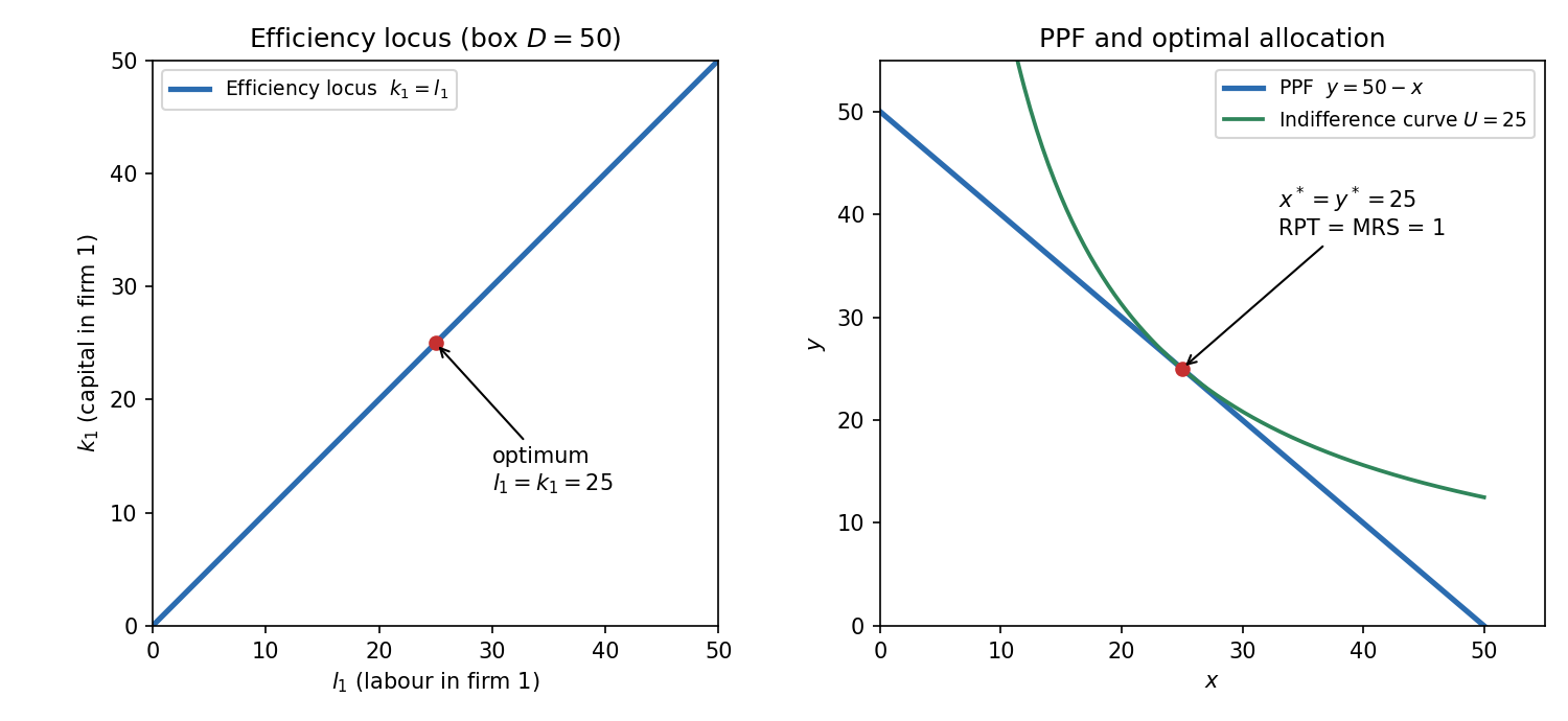
Left: the efficiency locus is the diagonal of the input box, and the optimum sits in the middle at . Right: the straight-line PPF is tangent to the indifference curve (utility ) at , where .
2d — A higher (2 points)
AnswerNothing changes: the quantities and the ratio stay the same.
The efficiency locus does not contain at all, and with the outputs on the locus are still and . So the PPF, the optimum, and are unchanged.
Intuitionchanges how much firms rely on labour versus capital, but both firms share it, and the total supply of the two inputs is the same ( each). On the diagonal the two inputs are used in equal amounts, so the labour share parameter never matters.
2e — A higher (2 points)
AnswerThe ratio rises.
Now : the PPF has a steeper slope () and a higher -intercept (). The optimum needs , so with the ratio equals and is higher.
IntuitionChecking the numbers myself: and give and . So with , the quantity of stays at 25 and the quantity of grows with , which is why the ratio grows. This is my own check, the official solution states only the direction of the ratio.
2f — A higher (2 points)
AnswerThe ratio falls: the consumer spends a larger share on and a smaller share on .
IntuitionThe condition with gives , so , which falls in . On the PPF this gives and : more , less . Again my own check of the official direction.
2g — A higher (2 points)
AnswerThe ratio is unchanged; quantities of both goods rise.
The efficiency locus and the RPT do not depend on , so the ratio is the same. The PPF shifts outwards (income rises) and both quantities rise in the same proportion.
IntuitionWith constant returns, doubling the resources doubles output of everything along the ray with the same ratio. Using the same working, .
Q3 — Partial equilibrium, subsidy and price cap (25 points)
Quasilinear consumer ( is money, no corner solutions). Firm with .
NumberingThe exam labels the last part (e), there is no (d); the official solution calls it (d). They are the same question (subsidy versus price cap).
3a — Cost function (8 points)
Answer
Working. Cost Minimisation: set the RTS equal to the input price ratio:
Plug into the isoquant for output :
Supply is marginal cost: .
3b — Equilibrium price and quantity (7 points)
Answerand .
For a Quasilinear Utility consumer, demand is marginal utility of (the marginal utility of money is 1):
3c — Consumer subsidy of 20 (5 points)
Answer
- and firm surplus .
- Government pays .
- Added welfare is , so the gain does not cover the cost (net loss of ).
Before the subsidy (Consumer Surplus and Firm Surplus):
After the subsidy. The official solution adds the subsidy to the demand curve, (the price the producer effectively receives is the consumer's willingness to pay plus 20):
IntuitionHere "60" is the price the firm receives; the consumer pays (the point on the original demand curve at ). The consumer surplus calculated with against the price 60 equals the surplus on the original demand against the price 40, so the same 900. The net loss of is the standard deadweight triangle: , because the subsidy pushes past the efficient quantity where value (marginal utility at ) falls below marginal cost ().
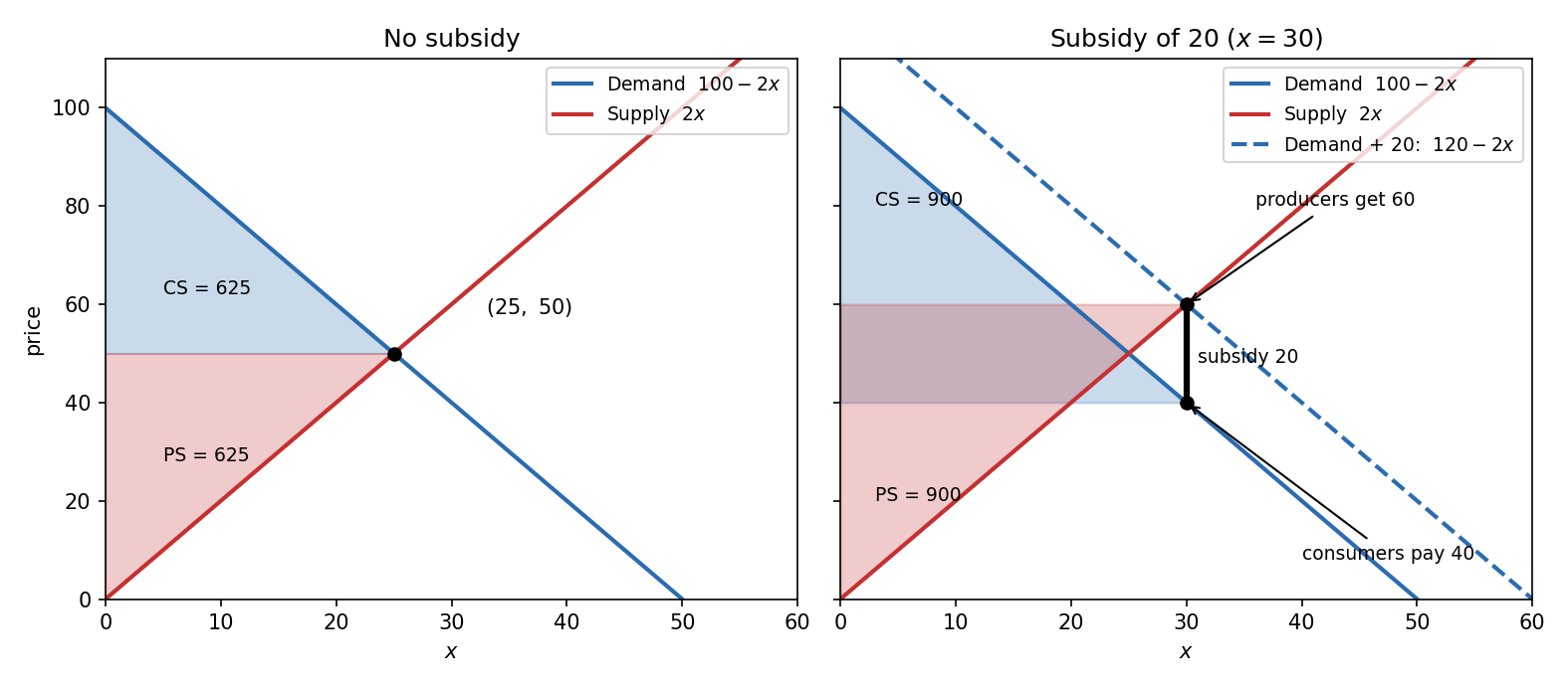
Left: surpluses at the competitive equilibrium. Right: with the subsidy, producers receive 60 and consumers pay 40 at ; each surplus rises from 625 to 900.
3d — Which policy gives higher welfare? (5 points)
AnswerThe subsidy gives higher welfare: (price cap at 10).
Price cap at 10. At price supply is , so only is produced, and demand exceeds supply (excess demand). Quantity is the short side, supply. Welfare is total value minus cost on the units traded:
Subsidy. Welfare is the surplus gain less the cost of the subsidy: .
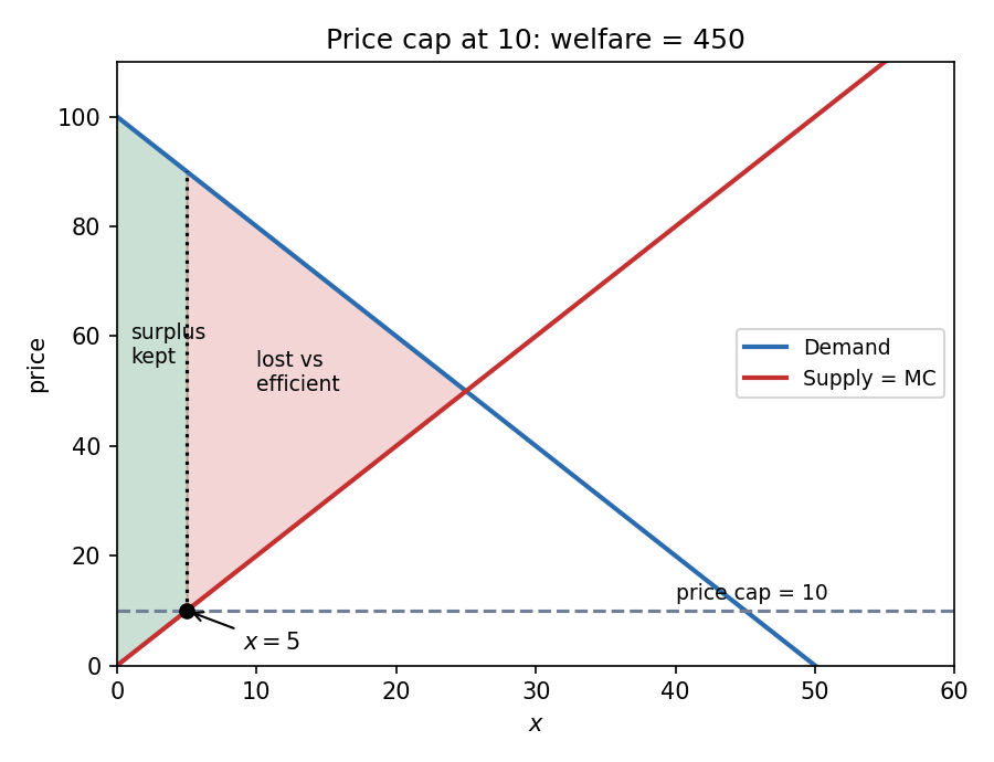
Under the cap at 10 only 5 units are traded; the shaded green area is the of welfare kept, and the large red triangle is the surplus lost compared with the efficient quantity.
IntuitionThe price cap is far below the equilibrium price of 50, so it chokes supply down to 5 units (against an efficient 25). The subsidy overshoots to 30, but the overshoot costs only a small triangle of 50 compared with the efficient welfare of 1,250.
Assumption in the official welfare of 450The figure treats the 5 units as going to the consumers who value them most (efficient rationing). With random queuing the welfare would be even lower, so the ranking does not change.
Recap table
| Part | Tool | One-line answer |
|---|---|---|
| 1 | Contract curve shifts when changes | True |
| 2 | Homogeneity needs both prices scaled | False, profit is divided by in the example |
| 3 | Quasilinear: | False, at low output labour rises |
| 4 | Strictly convex cost, | True, interior optimum |
| 5 | Cost minimisation uses only price ratio | True |
| 6 | Collinear bundles on one isoquant | False (key marks both words) |
| 7 | Two different dots, resources wasted | False |
| 8 | Planner with increasing | True |
| 9 | RTS equal only at the efficient input split | False |
| 10 | Lump-sum tax does not change margins | False |
| 2a | ||
| 2b | Outputs on the locus | |
| 2c | ||
| 2d | not in the locus | No change |
| 2e | RPT | rises |
| 2f | falls | |
| 2g | Scale economy | Ratio same, quantities up |
| 3a | RTS = price ratio | |
| 3b | , | |
| 3c | Shift demand up by 20 | , , cost 600, net |
| 3d | Welfare under a cap | , subsidy better |
Related notes
- Micro-Economics II (hub)
- Lec_04-Theory of the Firm, Partial & General Equilibrium
- Lec_05-Production Economy & Externalities
- PS_01-Profit Maximisation & Properties of the Profit Function
- PS_02-Isoquants, RTS & Properties of the Profit Function
- PS_03-Cost Minimisation & Properties of the Cost Function
- PS_04-Partial Equilibrium, Welfare & Price Ceilings
- PS_05-Pareto Efficiency, Dominance & Social Welfare
- PS_06-Exchange Equilibrium, Walrasian Prices & the Social Planner
- PS_08-Production Economy, Efficiency Locus & Input Allocation