
Cost Functions, Exchange Equilibrium, Price Cap & Public Good Provision (2024 Moed B)
- #microeconomics
- #past-paper
- #worked-solution
- #cost-function
- #corner-solution
- #exchange-economy
- #contract-curve
- #price-ceiling
- #public-goods
- #nash-equilibrium
Cost Functions, Exchange Equilibrium, Price Cap & Public Good Provision (2024 Moed B)
Part of: Micro-Economics II Micro 2 Final Exam, Moed B (April 2024), Micro-Economics II, Dr. Boaz Zik. 3 hours, open material, 4 questions, 25 points each. Builds on: Lec_04-Theory of the Firm, Partial & General Equilibrium, Lec_05-Production Economy & Externalities, Lec_06-Public Goods & Altruism Practice: PS_03-Cost Minimisation & Properties of the Cost Function, PS_04-Partial Equilibrium, Welfare & Price Ceilings, PS_06-Exchange Equilibrium, Walrasian Prices & the Social Planner
SourceAnswers follow the official solution (8 pages). Where the official text has a typo or a gap, the answer is kept and a
> [!warning]callout says so. Part 4d has no worked official solution.
What this paper tests
| Question | Core idea | Where it is taught |
|---|---|---|
| Q1 | Cost Minimisation with a technology that mixes a concave input and a linear input: a kinked Cost Function, and when the two-input firm is cheaper than the one-input firm | PS_03-Cost Minimisation & Properties of the Cost Function, Lec_04-Theory of the Firm, Partial & General Equilibrium |
| Q2 | Exchange Economy with Cobb-Douglas agents: Contract Curve, Walrasian Equilibrium, and what happens when agent 2's utility is scaled by | PS_06-Exchange Equilibrium, Walrasian Prices & the Social Planner |
| Q3 | Partial Equilibrium with Quasilinear Utility and a maximum price (Price Ceiling): welfare effects, then shifts in demand and in costs under a binding cap | PS_04-Partial Equilibrium, Welfare & Price Ceilings |
| Q4 | Public good with square-root benefits: stand-alone provision, social optimum, Nash equilibria, free riding | Lec_06-Public Goods & Altruism |
Intuition: the one move behind each question
- Q1: compare marginal product per dollar of each input. Labour is used first (its marginal product falls), capital takes over once labour's marginal product per dollar has dropped to capital's.
- Q2: identical Cobb-Douglas exponents mean identical MRS at any common ratio , so the contract curve is the box diagonal. Scaling a utility function by changes nothing real.
- Q3: under a binding cap, the quantity is set by the supply side ( equals the cap). Everything that does not move leaves quantity unchanged.
- Q4: each player equates her own marginal benefit to the price; the planner equates the sum.
Q1 — Cost functions with one and two inputs (25 points)
Input prices: , in parts a to c, then in part d.
1a — Cost function for (10 points)
Answer
Step 1: where does the firm switch inputs? The technology has Diminishing RTS in labour: falls with , while is constant. The Tangency Condition sets the RTS equal to the price ratio:
so , i.e. and .
Step 2: read off the two regimes. Labour alone can produce at most units while its marginal product per dollar is still at least capital's.
- If : use labour only, and . Cost .
- If : labour is held at the tangency level (which delivers units) and capital supplies the rest, . Cost .
IntuitionLabour is cheap but has diminishing returns, capital is dear but each unit always adds exactly one unit of output. The first units of output come from labour. Once labour's marginal cost has risen to (the cost of a unit of output via capital), the firm stops adding labour and buys capital. Check: for reaches at , and is ever after. The cost function is continuous at the kink: .
1b — Cost function for (5 points)
Answer
With one input there is no choice: gives and cost .
1c — When is the two-input firm strictly cheaper? (5 points)
AnswerFor all .
Compare the two cost functions from 1a and 1b:
- For they are identical, (the two-input firm chooses labour only, so it behaves like the one-input firm).
- For the difference is
so the two-input firm is strictly cheaper.
1d — The same question with , and the economics (5 points)
AnswerThe two-input firm is strictly cheaper for all (compare in part c).
Derivation. Tangency: , so , , . For use labour only (, cost ). For : , , cost . The gap is for .
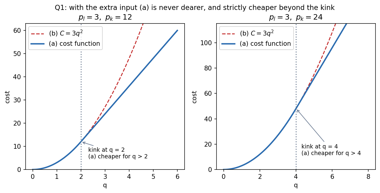
Left: , kink at . Right: , kink at . The dashed curve is the one-input cost . The two-input cost never lies above it and separates from it only after the kink.
Economic explanation (official)The quantity beyond which the two-input firm is cheaper depends on relative prices. The more expensive capital is, the later the firm moves from producing with labour to producing with capital, so the two-input firm has an advantage only at a larger quantity.
IntuitionCapital is a "backup" input. It only has value once labour has become expensive at the margin. If capital costs twice as much, labour must run twice as far up its marginal-cost curve ( must reach , not ) before capital is worth buying. So the kink moves from to .
Q2 — Exchange economy with a scale factor (25 points)
and . Total resources and .
2a — Numerical case: , , ,
Totals: .
(1) Contract curve (6 points)
Answer
On the Contract Curve, . Both agents have exponent and :
so . Cross-multiplying gives , so . The contract curve is the diagonal of the Edgeworth Box.
(2) Equilibrium prices and quantities (6 points)
Answer, , (good is the numeraire, ).
A Cobb-Douglas consumer spends the share of wealth on . Agent 1 has wealth :
Agent 2 has wealth :
Market clearing for , :
Then and . For : and . By Walras' Law the market clears too.
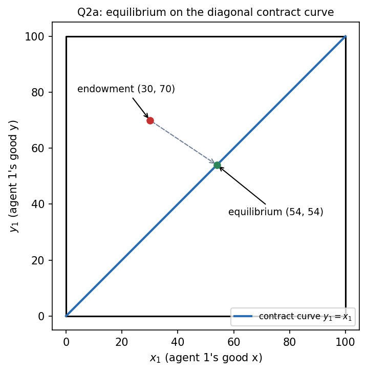
Trade moves agent 1 from the endowment to , which lies on the diagonal contract curve, as the First Welfare Theorem requires.
IntuitionAgent 1 starts with a lot of and little , agent 2 the reverse, and they have the same tastes. Trade moves them to the same bundle proportions. Agent 1 ends with slightly more than half of each good because is cheap relative to (), and agent 1 holds more -wealth: at these prices agent 1's wealth is against agent 2's .
2b — Equal split endowments: agent 2's utility is times agent 1's (7 points)
Endowments: .
AnswerThe equilibrium is at the endowment (no trade), so in equilibrium.
Why (official). Both agents hold the same bundle, and they have the same (the factor does not enter the , because it multiplies the whole utility function). So at the endowment : the endowment is already on the contract curve, and no mutually beneficial trade exists. The price ratio that supports it is the common , and each agent demands exactly her endowment. Then
IntuitionSame bundle plus same tastes means nothing to trade. The only difference between the agents is the scale factor , which multiplies utility but has no effect on choices.
2c — Moving from to with (6 points)
AnswerThe equilibrium allocation does not change. It is the endowment under both values of .
Why (official). Part (b) holds for any , and the does not depend on . So the equilibrium is at the common endowment whether or . Only the utility level of agent 2 changes (it scales up with ); the allocation and prices stay the same.
IntuitionUtility is ordinal. Multiplying a utility function by a positive constant represents the same preferences, so demands, prices and allocations are unaffected. Agent 2 is "happier" in only in the sense of the number attached to the same bundle, which has no economic meaning by itself. (It would matter for a social planner who adds utilities, as in PS_07-Core, Corner Endowments & Equilibrium vs the Social Planner.)
Q3 — Partial equilibrium and a maximum price (25 points)
Demand comes from a representative consumer with Quasilinear Utility (income high enough for an interior solution). Supply comes from a representative firm with and input prices , .
Setup used in every partFor quasilinear utility, the inverse demand equals the marginal utility of : . The inverse supply is the marginal cost, . Surplus formulas: and .
3a — ,
(i) Cost function (4 points)
Answer
Tangency: , so . The isoquant is , so and
The marginal cost is .
(ii) Equilibrium and welfare (4 points)
Answer, , , , .
Inverse demand is . Set it equal to marginal cost, , so and .
(iii) A maximum price of 80 (4 points)
Answer, , , .
Equilibrium Cap of 80 Change Quantity 30 20 down 10 900 1600 up 700 1800 800 down 1000 2700 2400 down 300
The cap of 80 is below the equilibrium price 120, so it binds. At a price of 80 consumers want , i.e. , but the firm supplies only where , i.e. , . The quantity traded is the short side, supply: .
Typo in the official solutionThe official text calls the second expression "the consumer surplus" twice: it says "The consumer surplus equal " (this is the firm surplus, giving 800) and later "The consumer surplus decreased" (it means the firm surplus). The numbers (1600 and 800) and the direction of each change are right.
Explanation (official). The consumer surplus rises: the lower price compensates the consumer for the lower quantity. The firm surplus falls because both the quantity and the price fall. Social welfare falls because the allocation no longer coincides with the equilibrium allocation.
Intuition: where the lost welfare goesThe loss is the Deadweight Loss triangle between demand and marginal cost over the units from to : at demand is and , so the triangle is . Splitting it up: on the units still traded, the price drop transfers from firm to consumer. On the units no longer traded, the consumer loses and the firm loses . So changes by , by , and the net is . This treats the units as going to the consumers who value them most, as the official formula does.
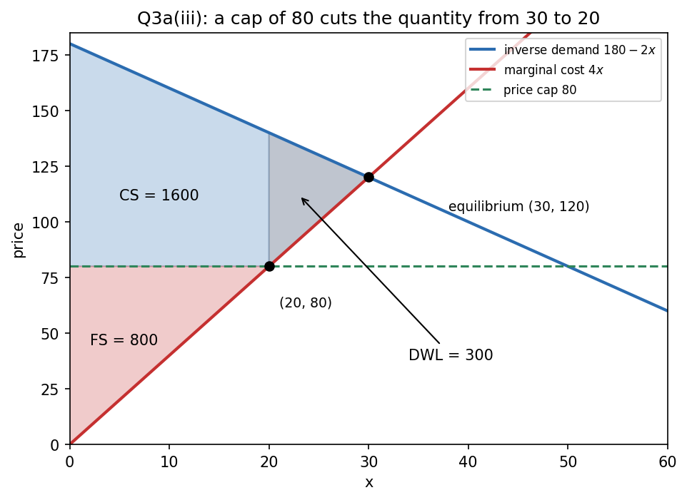
Blue: consumer surplus with the cap. Red: firm surplus with the cap. Grey: the deadweight loss triangle, units 20 to 30.
3b — Demand rises ( increases) under a binding cap (5 points)
AnswerThe firm surplus is unchanged. The consumer surplus rises.
Why (official). A higher shifts demand out, so the equilibrium price rises and the cap is still below it. The cap still binds, so the quantity is set where equals the cap. does not depend on , so the quantity is unchanged, and so is the price (it is the cap).
- Firm surplus : , and are all unchanged, so it does not change.
- Consumer surplus : and are unchanged, but is larger, so it rises by .
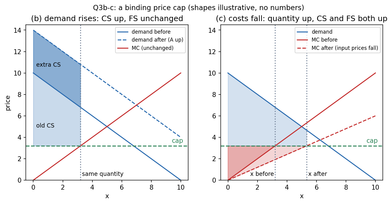
Left panel: demand shifts up, the quantity stays at the same point (set by the cap meeting MC), so the shaded consumer-surplus area grows while the firm's triangle does not move. Shapes are illustrative; no numbers are implied.
IntuitionThe consumer values every unit more, but the firm will not supply any more at a price of the cap. So the consumer enjoys a bigger gain from the same units. The extra demand only produces a bigger shortage.
3c — Input prices and fall under a binding cap (5 points)
AnswerThe quantity rises, the price stays at the cap, and both the consumer surplus and the firm surplus rise.
Why (official). A fall in input prices lowers the marginal cost curve. The quantity is where equals the cap, so it rises. The price stays equal to the cap.
- Consumer surplus: for a given price it increases in the quantity, so it rises.
- Firm surplus: the marginal cost has decreased, so the firm earns more on the same price and sells more, so it rises.
Intuition: a quick check with this firm's costs (mine)With where (the general version of part a(i)), the firm supplies and earns . A lower raises both the quantity and . The result needs the cap to still bind after the fall: if costs fell so far that the equilibrium price dropped below the cap, the cap would stop mattering. The question says the cap is kept, so we assume it still binds.
The right panel of the figure above shows the downward shift in and the larger quantity.
3d — How (b) and (c) differ (3 points)
Answer (official)In (b), demand rose. With a maximum price the quantity is set by supply, which did not change, so only the consumer benefits. In (c), costs fell, which increases supply, so the quantity changes and both the firm and the consumer benefit.
IntuitionUnder a cap the short side of the market is demand-heavy: there is a shortage. In a shortage the side that is not rationed (the supply side) decides the quantity. Shocks on the demand side just make the shortage bigger. Shocks on the supply side are the ones that actually change what gets traded.
Q4 — Public good provision (25 points)
Alice has utility and Bob has utility , where is the total public good and is money. Both have the same income (large enough never to bind). One unit of costs dollar. See Public Goods and Lec_06-Public Goods & Altruism.
4a — Provision when the other contributes nothing (5 points)
AnswerAlice buys (with ). Bob buys (with ).
A buyer stops where her marginal utility from the public good equals its price. For Alice, with Bob buying nothing:
For Bob, with Alice buying nothing:
4b — : optimum, equilibria and efficiency (7 points)
Answer
- Social optimum: .
- Nash equilibria: all pairs with .
- Level of : in equilibrium, which is less than the optimum of .
- Efficiency: the equilibrium is inefficient (under-provision).
Social optimum. The planner equates the sum of marginal utilities to the cost:
Nash equilibria. From part (a), each player alone wants a total of . If the other contributes , Alice tops up to reach a total of (or contributes nothing if ):
At any pair with , and , so each choice is a best response to the other. These are all Nash equilibria, and the total is in each.
Why they differ. Each player compares her own marginal utility with the cost and ignores the benefit her contribution gives the other player (a positive externality). The planner counts both benefits. The equilibrium total of is a quarter of the efficient .
Intuition (mine): the welfare loss in numbersTotal surplus from a total of is ( for the two players, minus the cost of ). At it is . At it is . The market equilibrium leaves units of surplus on the table, which is why it is not Pareto efficient: a move to with a suitable split of the cost can make both players better off.
4c — , : a unique equilibrium where only Bob contributes (5 points)
AnswerThe only Nash equilibrium is .
By 4a, Alice alone wants a total of and Bob wants a total of . The best responses are:
Showing uniqueness.
- Candidate . Bob's best response to is . Alice's best response to is . Each is a best response, so is a Nash equilibrium.
- No equilibrium with . Alice contributes only if , and then , so the total is . But then Bob, who wants a total of and so contributes , cannot be playing . Contradiction.
- Hence , and Bob's best response is . This is the unique equilibrium.
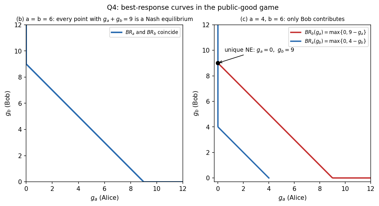
Left: with the two best-response curves coincide along , giving a continuum of equilibria. Right: with , the curves cross only where Alice contributes nothing, at .
IntuitionBob wants a total of ; Alice only wants a total of . Once Bob has bought , Alice's wish is already met, so she free rides. The one with the stronger taste for the good () provides it all.
4d — Verbal explanation of under-provision and free riding (8 points)
No official solutionThe official solution only says "See the discussion in class." No worked answer is given, so none is written here. The discussion it points to is in Lec_06-Public Goods & Altruism, Part 3c (the Nash equilibria by case) and Part 3d ("Why the Market Under-Provides"), with the results Under-Provision and Free Riding. Parts 4b and 4c above are the numerical examples of those two results.
Recap table
| Part | Tool | One-line answer |
|---|---|---|
| 1a | Tangency , then split at the kink | for ; for |
| 1b | One input, no choice | |
| 1c | Compare 1a and 1b | Two-input firm strictly cheaper for |
| 1d | Same with | for ; for ; cheaper for ; dearer capital delays the switch |
| 2a1 | ||
| 2a2 | Cobb-Douglas demands plus market clearing | ; agent 1 gets , agent 2 gets |
| 2b | Same bundle, same , so no trade | Equilibrium at the endowment, |
| 2c | is independent of | Allocation unchanged when goes from to |
| 3a(i) | RTS = price ratio, so | |
| 3a(ii) | , , , , | |
| 3a(iii) | Cap binds, quantity from | , , , |
| 3b | Quantity set by cap, which does not move with | unchanged, up |
| 3c | falls, so quantity at the cap rises | and both up |
| 3d | Supply side decides quantity under a cap | (b) only consumers gain; (c) both gain |
| 4a | Own marginal utility = 1 | Alice ; Bob |
| 4b | Sum of marginal utilities = 1; best responses | Optimum ; Nash: ; under-provision |
| 4c | Best responses , | Unique Nash equilibrium |
| 4d | Class discussion | No official solution |
Related notes
- Micro-Economics II (hub)
- Lec_04-Theory of the Firm, Partial & General Equilibrium
- Lec_05-Production Economy & Externalities
- Lec_06-Public Goods & Altruism
- PS_03-Cost Minimisation & Properties of the Cost Function
- PS_04-Partial Equilibrium, Welfare & Price Ceilings
- PS_06-Exchange Equilibrium, Walrasian Prices & the Social Planner
- PS_07-Core, Corner Endowments & Equilibrium vs the Social Planner