
Finance Cheat Sheet
- #financial-management
- #fundamentals-of-finance
- #reading
- #formula-sheet
- #time-value-of-money
- #bonds
- #loans
- #capital-budgeting
- #portfolio-risk
- #capm
Finance Cheat Sheet
Part of: Financial Management Reading 1 — Financial Management & Finance Source:
Finance Cheat Sheet.pdf(4 pages, Amitai Malik, Teaching Success)
This is a summary sheet, not a taught lessonIt is the course formula sheet: every formula the course uses on four pages, with a few worked examples. It sits under Readings on the site. Use it to revise and look up formulas; to learn a topic, follow the link in each section to the lesson that teaches it. The sheet has two blank "Personal Additions" boxes, which are not reproduced.
How the sheet is organisedIt follows the course order: #1. Time value of money, #2. Interest rates: stated vs effective, #3. Inflation and the Fisher equation, #4. Bonds, #5. Loans, #6. Project choice: NPV, IRR and friends, #7. Risk and reward (the part with no lesson), then #8. Capital budgeting: free cash flow.
1. Time value of money
Taught in Lesson_01-Time Value of Money and Lesson_02-Perpetuities, NPV & IRR. Practice: HW_01-Time Value of Money.
is the discount rate and, unless the question says otherwise, it is compounding.
- Discounting = moving to the left on the timeline: divide by .
- Compounding = moving to the right: multiply by .
Here is the number of periods (or payments, for annuities), the periodic payment, the periodic growth rate.
| Cash flow | Present value | Future value at |
|---|---|---|
| Single cash flow | ||
| Annuity (finite, identical payments) | ||
| Growing annuity | ||
| Perpetuity (infinite, identical payments) | none | |
| Growing perpetuity | none |
Two timing rules from the sheet
- PV takes you one period before the first payment.
- FV takes you to the final payment.
Plain English. The PV of an annuity is "payment divided by the rate, minus the part that would have been paid after year ". A growing perpetuity is the same idea with the rate reduced by the growth.
Special cases and tools:
When growth equals the discount rate, every payment has the same present value, so the PV is just equal pieces.
The -th payment of a growing stream.
A growing perpetuity only has a finite price if .
Extracting the power (solving for ): if , then
Take logs of both sides to bring down from the exponent.
Excel: PV, FV, PMT, NPER and RATE cover the annuity rows; for a stream of different amounts use NPV.
2. Interest rates: stated vs effective
Taught in Lesson_03-Rate Conversion, Effective Rates & EAC. Practice: HW_04-Effective Interest Rates.
Three ground rules from the sheet: always draw a timeline; adjust every rate to the same period as the timeline (monthly payments need a monthly rate); and when comparing scenarios, find each one's PV and compare.
= how many times the shorter period fits into the longer one.
| To the shorter period | To the longer period | |
|---|---|---|
| Stated interest (APR) | ||
| Effective interest (EAR) |
Stated rates are split or multiplied; effective rates are compounded or rooted. See Stated Rate and Effective Interest Rate.
When stated and effective differ
The sheet lists three situations.
1. Interest compounded more than once a period ( = number of compoundings):
Example from the sheet: APR compounded monthly gives
2. Interest paid in advance ( = the transaction's length):
You receive less than you borrow, so the true rate is higher than the stated one. Example: APR , one year, paid in advance:
Sheet roundingThe sheet prints . The exact value is , which rounds to . The sheet truncated it.
3. Commissions. Draw the timeline, then solve the equation below for , discounting with itself:
Example from the sheet: a $100 loan for one year at APR plus a $4 commission paid at expiry. At time 1 you pay back :
3. Inflation and the Fisher equation
Taught in Lesson_04-Inflation, Real Rates & Expected Inflation. Practice: HW_05-Inflation & Real Annuities.
is periodic inflation. Actual inflation from time 0 to , from a price index or from period inflations:
Cumulative inflation is a ratio of price levels, or a product of the yearly growth factors. Never a sum.
Sheet examples:
- Base index , : . If : .
- Yearly inflations : .
Index-linked vs non-index-linked
| Real value (without inflation) | Nominal value (money in our pocket) | |
|---|---|---|
| Index-linked (real rate; compensates for time and risk only) | ||
| Non-index-linked (nominal rate; compensates for time, risk and expected inflation) |
Which is better, in the sheet's words:
- If (actual below expected), non-index-linked is better. If , index-linked is better.
- Non-index-linked is more dangerous: we cannot know whether we will withstand future payments.
Fisher equation
Nominal growth = real growth times expected price growth. See Fisher Equation. Two conditions: all variables must cover the same time period, and all must be effective (not stated) rates.
Worked example from the sheet. A bank offers a quarterly effective 3% on index-linked deals and a semi-annual effective 10% on non-index-linked deals. What annual inflation does the bank expect? First put both on the annual period:
Then plug into Fisher:
4. Bonds
Taught in Lesson_07-Bond Pricing. Practice: HW_08-Bond Pricing.
Notation: = coupon rate (stated), = market rate (effective), = face value, = the bond's price, = coupons per year, = number of coupons.
First step in every bond question: find the coupon. See Coupon and Face Value.
Classic bond (equal coupons, at maturity), price at issuance:
An annuity of coupons plus the discounted face value.
Zero-coupon bond (Zero-Coupon Bond), and coupons in perpetuity (no ):
Price after issuance, coupons already paid:
Just before a coupon is handed out, you still get it, so add one more .
Discount, par, premium (see Yield to Maturity):
| Issued at | Condition |
|---|---|
| Discount | , so |
| Par | , so |
| Premium | , so |
Credit rating. Safer bond, higher rating, lower market rate, higher price. Dangerous bond, lower rating, higher market rate, lower price.
Worked example from the sheet. 3-year bond, annual 10% coupons, . 30% of is repaid at the end of year 1, the rest at maturity. . Cash flows (this is not a classic bond, so discount each flow):
| Time | Coupon | Principal repaid | Total |
|---|---|---|---|
| 1 | |||
| 2 | none | ||
| 3 |
Excel: PV prices a classic bond; for irregular cash flows discount each flow with NPV; RATE or IRR recovers the YTM from a price.
5. Loans
Taught in Lesson_05-The Four Loan Types. Practice: HW_06-Loans & Amortization.
Notation: = starting balance at time , = interest rate, = number of payments, and for period : = principal part, = interest part, = payment.
Annuity loan (Spitzer loan): constant payment
First step: find the payment from
Amortization row for period :
| Starting balance | Payment | Interest | Principal | Ending balance |
|---|---|---|---|---|
Totals and a useful pattern:
In a Spitzer loan the principal repaid grows by a factor each period.
Regular loan: constant principal
First step: the periodic principal.
| Starting balance | Principal | Interest | Payment | Ending balance |
|---|---|---|---|---|
Payments shrink each period because interest falls with the balance.
Bullet loan and balloon loan
Bullet (Bullet Loan): one single payment at the end.
Balloon: periodic interest-only payments, then the whole principal at the end.
Index-linked vs non-index-linked loans
- For an index-linked loan, multiply the result by actual inflation to get the nominal value.
- A non-index-linked loan already contains the nominal rate (with expected inflation inside), so multiply by nothing at the end.
Excel: PMT, IPMT, PPMT, PV, RATE.
6. Project choice: NPV, IRR and friends
Taught in Lesson_02-Perpetuities, NPV & IRR (NPV, IRR), Lesson_03-Rate Conversion, Effective Rates & EAC (profitability index, EAC) and Lesson_06-Capital Budgeting & Free Cash Flow. Practice: HW_02-NPV, IRR & Project Choice, HW_03-Profitability Index & EAC.
The two defining formulas:
Net Present Value is today's value of all the cash flows; the Internal Rate of Return is the discount rate that makes it zero. Excel: NPV (remember it starts at period 1, so add separately), IRR.
The decision tree on the sheet
| Situation | Rule |
|---|---|
| Single project, NPV test | : accept. : indifferent. : reject. |
| Single project, IRR test (only if the project is standard) | : accept. : indifferent. : reject. |
| Multiple, mutually exclusive | Pick the greatest NPV, or the greatest (below). |
| Multiple, not mutually exclusive, unlimited budget | Undertake every project with . |
| Multiple, not mutually exclusive, budget constraint, partial projects not allowed | Choose the combination with the greatest cumulative NPV. |
| Multiple, not mutually exclusive, budget constraint, partial projects allowed | Rank by profitability index . |
| Renewable projects with unequal lives, or continuous projects | Pick the greatest (below). |
When the IRR test is safeThe sheet says to use the IRR rule only if the project is "standard" (one sign change in the cash flows: outflow first, then inflows). For non-standard projects, trust NPV.
Modified IRR (Modified Internal Rate of Return):
Compound all inflows forward to the end, discount all outflows back to today, and take the single-period growth rate between them.
Equivalent annual value (Equivalent Annual Cost is the cost-side version), for projects with unequal lives:
Turn each project's NPV into a level yearly amount over its own life, so projects of different lengths become comparable.
7. Risk and reward
No lesson in this course covers this sectionThe course has no lesson on risk, return, portfolios, beta or the SML. The only note that practises it is HW_09-Risk, Return & Diversification, so treat this sheet as the main source for the formulas and the homework as the worked practice. Plain-English glosses below are mine; the formulas are the sheet's.
Learning order that makes this section easy: (a) one asset, (b) two or three assets, (c) add a risk-free asset, (d) market portfolio and the CML, (e) beta and the SML, (f) split total risk into market and specific.
7.1 One asset
Based on scenarios, where is the scenario's probability and the asset's return in that scenario:
Expected return is the probability-weighted average; variance is the probability-weighted squared distance from it. See Expected Return.
Based on historical data ( observations):
With history, use the plain average and divide the variance by (not ).
7.2 Two assets
are the investment proportions and must add to 1:
Correlation measures how the two returns move together (Correlation):
| Covariance | Correlation |
|---|---|
| (move together) | |
| (unrelated) | |
| (move opposite) |
Portfolio expected return and variance (Portfolio Risk):
The return is a plain weighted average, but the risk is not: the cross term shrinks as falls, which is the whole point of Diversification.
For three assets (, , ):
Every asset's own variance, plus twice every pair's covariance term.
7.3 Minimum variance portfolio (MVP)
The mix of and with the lowest possible risk (Minimum Variance Portfolio). The sheet gives the general formula for (it also reproduces the two shortcuts below):
Shortcuts for the three standard cases:
| Case | MVP weight | What the curve looks like |
|---|---|---|
| Two straight lines meeting on the vertical axis: risk can be driven to zero | ||
| A curve bending back to the left of | ||
| A straight line from to : no diversification, so the MVP is simply the less risky asset |
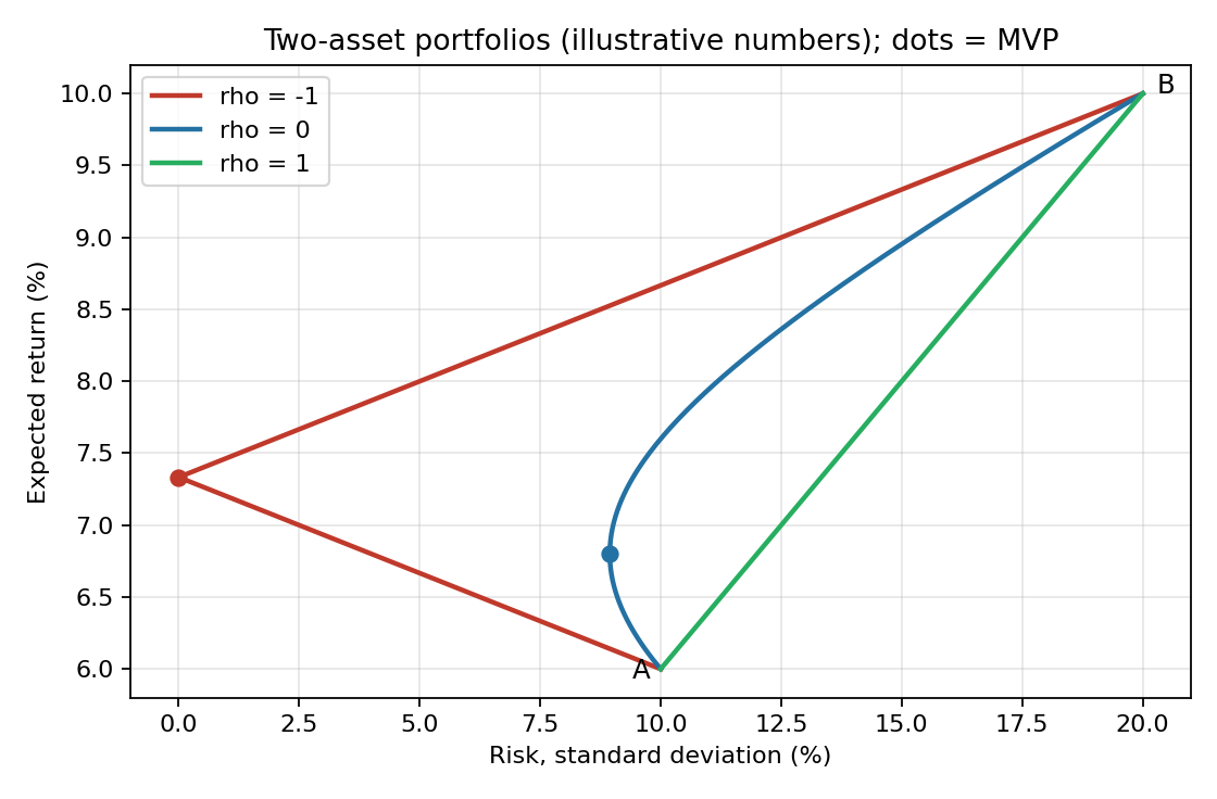
About this figureTheory diagram with illustrative numbers I chose (, , , ), not real data. It redraws the three small sketches on the sheet. The dots mark the MVP for (zero risk) and .
7.4 Adding a risk-free asset
With one risky asset and a risk-free asset :
The risk-free part has no variance and no covariance, so portfolio risk is just the risky share times the risky asset's risk.
Leveraged portfolio. The investor borrows at the risk-free rate to invest more than their own money, so :
The same formulas for and apply. Leverage raises expected return in exchange for higher risk.
Short selling is another way to lever up: sell one stock short to buy more of another.
Check: the weights still add to 1, the short-sold asset's weight is negative.
7.5 Efficient portfolio and the CML
An efficient portfolio combines the risk-free asset with the market portfolio (all risky assets in the market, held in proportion to their market worth).
- Step 1 is the same for every investor: determine .
- Step 2 is personal: choose how to split between and (the more risk averse, the closer to ).
Where an efficient portfolio sits:
| Position | Weights |
|---|---|
| On | |
| Between and | |
| On | |
| Right of (leveraged) |
The Capital Market Line (Capital Market Line) links an efficient portfolio's expected return to its risk. Always leave and as variables:
Start at the risk-free rate and add the market's extra return per unit of risk, times the risk you take.
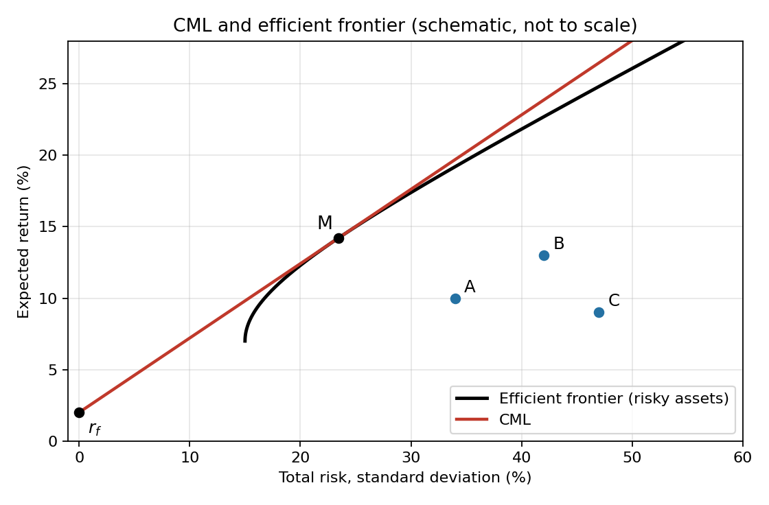
About this figureTheory diagram, schematic and not to scale; the shapes are mine, redrawing the sheet's page-4 sketch. The CML touches the efficient frontier of risky assets at . , , are single assets that sit below the CML.
7.6 Inefficient portfolios, beta and the SML
A portfolio that is not a mix of the risk-free asset and the market portfolio is inefficient. Single assets and inefficient portfolios are priced by the Security Market Line (Security Market Line), which fits all portfolios and assets:
Required return = risk-free rate + market risk premium times the asset's sensitivity to the market.
- The risk premium is .
- If you are given , always use the SML, even for an efficient portfolio.
- The from the SML can be used as the discount rate: .
Beta (Beta) is how sensitive an asset is to market moves.
- Rule 1: the greater the , the more sensitive the asset, the higher the return investors demand.
- Rule 2: the market portfolio has , and a risk-free asset has .
A portfolio's beta is the weighted average of its parts' betas, and an efficient portfolio's beta is just its share in the market portfolio, because the risk-free part has beta 0.
Regression form ( are the actual returns of asset , the risk-free asset and the market):
is the part of 's return that is not related to the market.
7.7 Market risk vs specific risk
Total variance splits into the part driven by the market (systematic, undiversifiable) and the part unique to the asset (specific, also called diversifiable, unsystematic or idiosyncratic). See Systematic Risk and Idiosyncratic Risk.
7.8 Reading the CML / efficient-frontier diagram
The sheet's last diagram (page 4) puts risky assets around the efficient frontier. Its bullet points:
- is where and : the intersection of the CML and the efficient frontier of all risky assets.
- The market portfolio contains all risky assets in proportion to their market worth. , , are points on the SML.
- (total risk of ) = market risk (undiversifiable) up to the CML, plus specific risk (diversifiable) from the CML to .
- The closer an asset is to the CML, the better its correlation with the market. The gap between the asset and the CML is (epsilon).
Comparing assets and (the sheet's example):
| Comparison | Answer |
|---|---|
| Identical total risk () | Same distance from the vertical axis |
| Greater market risk | (further from the axis, up to the CML) |
| Greater specific risk | (further from the CML) |
| Greater correlation with the market | () |
8. Capital budgeting: free cash flow
Taught in Lesson_06-Capital Budgeting & Free Cash Flow. Practice: HW_07-Free Cash Flow & Project NPV.
Steps to solve a capital budgeting question: (1) analyse the information; (2) build a final table with all the project's variables; (3) find the NPV to judge profitability.
Straight-line depreciation (Depreciation):
The free cash flow table
Rows, from top to bottom (Free Cash Flow), one column per time :
| Row | |
|---|---|
| + | Revenues |
| − | Expenses |
| − | Depreciation |
| = | Operational Profit (EBIT) |
| − | Corporate tax expenses |
| = | Net Operating Profit after Tax (NOPAT) |
| + | Depreciation (add back, it is not a cash cost) |
| + | Tax-free revenues |
| − | Undeductible expenses |
| − | Cost of project or initial investment |
| + | Money received for the sale of fixed assets |
| − | Capital gains tax for the sale of fixed assets |
| − | Changes in working capital |
| = | Free Cash Flow |
Rules the sheet attaches to the table:
- Any revenue or expense is taxable unless noted otherwise.
- If there are several revenues or expenses, each goes on a separate row.
- Sometimes irrelevant information is given and must be ignored:
- A. Sunk costs: an expense that has already happened or was already promised in the future.
- B. Funding (loans, bonds) and financing expenses.
- C. Payroll: if the existing workforce is used with no addition to their pay, ignore their wages; if there is an increase in their wages due to the project, count it as a project cost.
- General rule when information is misleading: what happens with the project minus what happens without the project is what goes in the table.
Sale of fixed assets
Sometimes equipment is sold before it is fully depreciated. The accounting (book) value differs from the sale price, and the gain is taxed.
Worked example from the sheet. A mining company buys tractors for $500,000 for a project, depreciated over 5 years with no salvage value. After 3 years they are sold for $300,000. Capital gains tax is 20%.
In the table: +$300,000 (sale proceeds) and −$20,000 (capital gains tax). The company is left with $280,000.
Investment in working capital
Working capital is the cash tied up in running the business day to day:
Inventory is stock not yet sold, customers is what customers still owe you, suppliers is what you still owe. See Working Capital.
The change in working capital is the row that goes in the free cash flow table (it is "part of the original table", the sheet stresses). An increase in working capital is a cash outflow; a decrease is an inflow.
Worked example from the sheet. "ABC Computers" just started. A customer buys a computer and pays $6,000 in 6 monthly installments; ABC buys the same computer from "HM" for $6,000 cash. So the owners must put in $6,000 of working capital at time 0, and take $1,000 out each month as the customer pays.
| Time | 0 | 1 | 2 | 3 | 4 | 5 | 6 |
|---|---|---|---|---|---|---|---|
| Inventory | 0 | 0 | 0 | 0 | 0 | 0 | 0 |
| Customers (still owed) | 6,000 | 5,000 | 4,000 | 3,000 | 2,000 | 1,000 | 0 |
| Suppliers (owed) | 0 | 0 | 0 | 0 | 0 | 0 | 0 |
| Working capital | 6,000 | 5,000 | 4,000 | 3,000 | 2,000 | 1,000 | 0 |
| Change in working capital | (6,000) | 1,000 | 1,000 | 1,000 | 1,000 | 1,000 | 1,000 |
General rule from the sheetThe sum of the changes in working capital must be zero at the end: all the cash tied up is eventually released. Use this to check your table.
Quick finder
| I need | Section | Lesson |
|---|---|---|
| PV or FV of a stream, solving for | #1. Time value of money | Lesson_01-Time Value of Money |
| APR to EAR, rates paid in advance, commissions | #2. Interest rates: stated vs effective | Lesson_03-Rate Conversion, Effective Rates & EAC |
| Real vs nominal, expected inflation | #3. Inflation and the Fisher equation | Lesson_04-Inflation, Real Rates & Expected Inflation |
| Price a bond or find the coupon | #4. Bonds | Lesson_07-Bond Pricing |
| Amortization tables, loan types | #5. Loans | Lesson_05-The Four Loan Types |
| Accept or reject, rank projects | #6. Project choice: NPV, IRR and friends | Lesson_02-Perpetuities, NPV & IRR |
| Portfolio risk, beta, CML, SML | #7. Risk and reward | no lesson; HW_09-Risk, Return & Diversification |
| Build a free cash flow table | #8. Capital budgeting: free cash flow | Lesson_06-Capital Budgeting & Free Cash Flow |