
Time Value of Money
- #financial-management
- #time-value-of-money
- #present-value
- #future-value
- #annuity
Time Value of Money
Part of: Financial Management Lesson 1 — Financial Management & Finance Key concepts: Time Value of Money, Future Value, Present Value, Discount Rate, Annuity, Growing Annuity
Why a dollar today beats a dollar tomorrow
The whole of corporate finance rests on one idea: a dollar today is worth more than a dollar tomorrow because today's dollar can be invested and earn a return. The Discount Rate is the exchange rate between money at different points in time. Everything else in this course — NPV, IRR, bond prices, loan schedules — is an application of moving cash flows along the time axis using .
The two operations
- Compounding pushes money forward in time: multiply by per period → Future Value.
- Discounting pulls money backward in time: divide by per period → Present Value.
Future Value & the power of compounding
Invest today at rate . After one period it grows to ; after periods each year's balance itself earns interest (interest on interest), so:
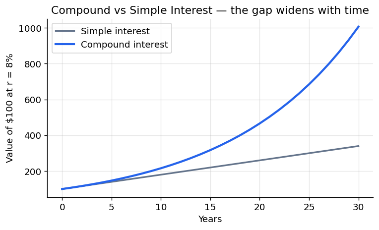
Compound ≠ simple interestSimple interest pays only on the original principal: . Compound interest pays interest on accumulated interest too: . Over short horizons the gap is tiny; over long horizons it explodes.
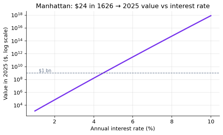
The Manhattan story — why the exponent dominatesLegend says Manhattan was bought in 1626 for t = 399$ years):
- Simple interest at 10%: — almost nothing.
- Compound interest at 10%: — astronomically more.
The lesson: at long horizons the value is hyper-sensitive to . Dropping the rate from 10% to 5% slashes the 2025 value by eight orders of magnitude.
Present Value & discounting
Reverse the FV formula. A cash flow arriving at time is worth, today:
Single cash flow$20{,}000 received in 2 years at : .
The PV of a stream of cash flows is just the sum of each flow discounted to today — this additivity is the value-additivity principle and it is what makes NPV work:
Excel
PV(rate, nper, pmt, [fv], [type])returns the PV of a level stream. Excel returns a negative number for a cash inflow (sign convention: money you receive is an outflow from the bank's view), so we often write-PV(...).
Annuities — a shortcut for level streams
An annuity is a finite stream of equal payments for periods. Rather than discount each one, use the closed form (derived by summing a geometric series):
Check, , : — identical to discounting all five payments individually. Excel:
-PV(5%,5,1000).
Ordinary annuity vs annuity-due
Timing matters
- Ordinary annuity (annuity-immediate): payments at the end of each period (). This is the default of the formula above and of Excel's
PV.- Annuity-due: payments at the start of each period (). Every payment is discounted one period less, so it is worth the ordinary annuity. Excel:
PV(rate,nper,pmt,,1)(the trailing1setstype = beginning).
Delayed (deferred) annuity
If the stream doesn't start until period , value it as an ordinary annuity as of one period before it starts, then discount that lump back to today.
Payments of $1000 in years 7–11,
- Value at : .
- Discount to : .
Growing annuity
When payments grow at rate each period — — the PV has its own closed form:
Check (lecture)(first payment), , , : PV — matches summing all twenty growing, discounted payments.
Intuition for in the denominatorGrowth partially offsets discounting. Only the net rate erodes value, so a faster-growing stream is worth more. If the finite formula still works, but a perpetual growing stream would diverge (see Lesson_02-Perpetuities, NPV & IRR).
Comparison table — the four building blocks
| Stream | Cash-flow pattern | PV formula | Excel |
|---|---|---|---|
| Single flow | one at time | =CF/(1+r)^t |
|
| Ordinary annuity | level , | -PV(r,n,C) |
|
| Annuity-due | level , | annuity | PV(r,n,C,,1) |
| Growing annuity | (no native fn) |
Summary
Key takeaways
- Compounding multiplies by ; discounting divides by it. They are inverses.
- PV is additive across cash flows — the foundation of NPV.
- Annuities and growing annuities are geometric-series shortcuts; learn both the closed form and the Excel function.
- At long horizons, value is dominated by the rate: small changes in produce huge changes in FV/PV.
- Watch the timing convention: end-of-period (ordinary) vs start-of-period (due) differ by exactly one factor of .
Related Notes
- Lesson_02-Perpetuities, NPV & IRR — extends annuities to infinity (perpetuities) and applies PV to project decisions
- Lesson_03-Rate Conversion, Effective Rates & EAC — what to use when compounding isn't annual
- Lesson_04-Inflation, Real Rates & Expected Inflation — nominal vs real discount rates
- HW_01-Time Value of Money — problem set applying every formula here
- Financial Management — subject hub