
Confidence Intervals & Change of Units
- #intro-econometrics
- #confidence-interval
- #standard-error
- #degrees-of-freedom
- #t-distribution
- #normality-assumption
- #change-of-units
- #OLS
Confidence Intervals & Change of Units
Part of: Intro Econometrics | Key concepts: Confidence Interval, Standard Error, Degrees of Freedom, Normality of Errors (A5), t-Distribution, Critical Value, Change of Units, Gauss-Markov Theorem
Where this lecture sits
Estimation to inferenceUp to now the course asked: given the data, which fits best? This lecture asks: how far from could the true plausibly be? The tool is the confidence interval, built from the standard error and the t-distribution. A second block shows how rescaling or changes the estimated coefficients. The same ideas are revised in Lec_13-Exam Review; worked practice is in Assign_01-Interpreting OLS Output & the Birthweight-Smoking Regression and Assign_03-Change of Variables, Regression Through the Origin & the Housing Model (answer keys: Assign_01-Solutions (Answer Key), Assign_03-Solutions (Answer Key)).
Short recap of last lecture (the deck opens with it):
- An estimator has a sampling distribution; it is unbiased if and efficient if it has the lowest variance among unbiased estimators.
- Gauss-Markov Theorem: if the model is linear and A1 to A4 hold, OLS has the smallest sampling variance of any linear unbiased estimator (BLUE).
- A1: . A2: (exogeneity). A3: for . A4: (homoskedasticity).
The new material has four parts:
- Estimating and the idea of degrees of freedom.
- Adding the normality assumption A5, so has a known shape.
- Building and interpreting confidence intervals, with two R examples.
- Change of units.
1. Estimating the variance of
The plan
- Use the residuals to estimate the error variance .
- Plug it into to get the Standard Error of .
- Use the standard error to build an interval where likely falls.
The variance formulas from last week contain the unknown :
Estimating
By definition (since ). We replace the unobservable error by the residual and the expectation by a sample average:
With explanatory variables ( parameters) divide by instead. Substituting gives the estimated variances and ; the standard error is the square root.
Why not divide by ?The residuals are not free: they must satisfy equations that the fitted parameters impose. Each parameter we estimate costs one degree of freedom, so dividing by the number of free residuals () corrects the bias.
Degrees of freedom
Degrees of Freedom = the number of observations (pieces of information) that are free to vary once a parameter that uses them has been estimated.
Heights (slide example)Sample of heights with known mean . Then can vary freely, but is forced. So the sample variance has 3 degrees of freedom: .
For regression the OLS first-order conditions are two equations that the residuals must satisfy:
Given these pin down (from the first) and (from the second). Two residuals are determined, so only are free.
Reconstructed from the slidesThe slide shows the two equations being solved for one residual each (slide 19). The summary sentence "two parameters estimated, so two degrees of freedom lost" is the slide's stated conclusion; the step-by-step wording above is mine.
2. The shape of the sampling distribution: assumption A5
To turn a standard error into an interval we need the shape of the distribution of . We add a fifth, weak assumption to A1 to A4:
A5: normality of the random errorsFor all : . See Normality of Errors (A5).
Why it makes normal
The key fact: a linear transformation of normal variables is normal. Activity 5 practises this: for with and ,
Reconstructed from the slidesThe slides pose the activity (slides 25 to 27) and leave the answers blank. The two results above are my working: expectation is linear and ; variance of a sum of uncorrelated terms adds, and constants drop out.
The slope estimator is a linear function of the errors:
So is a linear transformation of the normal errors, and the same holds for . Using the (already derived) mean and variance:
with , (slide 29 leaves these as fill-in boxes).
Standardising: Z then t
A normal standardises to . Applied to the slope:
This needs , which is unobserved. Replacing it with the estimate changes the distribution from normal to Student's t:
For the intercept the same recipe applies (Activity 5 part 2: divide by using the variance formula above).
| Standard normal | Student's | |
|---|---|---|
| Uses | true | estimated |
| Tails | thinner | "fatter" |
| Large | very close to | |
| Small | noticeably wider, reflecting the extra uncertainty from estimating |
IntuitionEstimating the variance adds noise, so we need more room in the tails. The fewer the degrees of freedom, the fatter the tails; with many degrees of freedom the t is almost normal.
3. Confidence intervals
Definition
- is fixed but unknown; almost surely. A Confidence Interval is an interval estimate (a point estimate is a single ): a lower bound and an upper bound computed from .
- Imagine drawing sample after sample. The 95% CI is the pair such that the true parameter lies inside for 95% of samples.
- In general a level CI satisfies
where is the significance level (usually 5%), the confidence level (usually 95%).
Interpreting a CIThe randomness is in the interval, not in . "95%" describes the procedure over repeated samples; for one realised interval, is either in it or not. The slides define it via repeated samples and do not discuss the one-sample reading.
Activity 5: the 100% intervalSince a normal (or t) variable ranges over , the only interval that is 100% certain is . Useless in practice: higher confidence means a wider interval.
Deriving the interval for an OLS coefficient
With estimated parameters, (for simple regression ). Let be the Critical Value that leaves area in each tail:
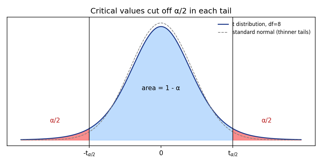
Substitute and rearrange the inequality to isolate :
Compactly:
NotationThe slides write throughout; in the R examples the number they plug in (e.g. 0.019) is the standard error column of
summary(), i.e. already the square root.
Getting the critical value
- From the t table: choose the degrees of freedom row () and the column for the significance level. The table is labelled by one-tailed and two-tailed levels; for a two-tailed CI use the two-tailed column (, , for 90%, 95%, 99%). If your exact df is missing, use the closest value (the slides use 30 for 32).
- In R:
qt(p = 0.975, df = 32)gives the 95% critical value (use ).
| Confidence | qt argument () |
(R, slide 52) | |
|---|---|---|---|
| 90% | 0.10 | 0.95 | 1.694 |
| 95% | 0.05 | 0.975 | 2.037 |
| 99% | 0.01 | 0.995 | 2.738 |
Activity 5 part 3: a hand calculation, (so 8 degrees of freedom), , so . The two-tailed 5% critical value at 8 df is , so the 95% CI is , i.e. . The common slip is to use the variance (4) instead of its square root (2).
Reconstructed from the slidesThe slides set up the problem (slides 45 to 47) and leave the answer box empty. The numbers above are my working with the table value for 8 df.
What makes a CI wide?
The interval is larger when:
- the standard error is larger, or
- the confidence level is higher (e.g. 99% rather than 90%).
The size of the estimate does not affect the width: the interval is always centred on .
Example 1: income-consumption model
Model: . Israeli macro data, yearly 1975 to 2008, per capita in NIS at 2005 prices. is the change in consumption per capita when GDP per capita rises by one shekel (the average marginal propensity to consume); is consumption at GDP of 0.
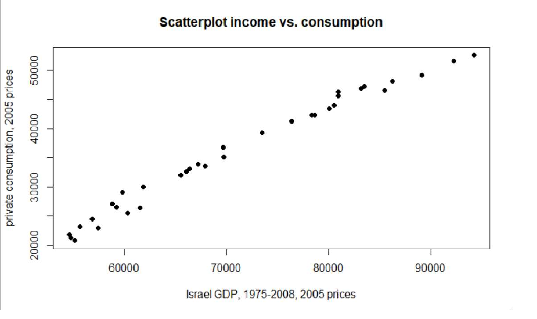
The relation looks linear. R output (summary(lm(cons.2005 ~ gdp.2005))), with the pieces needed for a CI highlighted on the slide: the estimates, the standard errors, and the degrees of freedom.
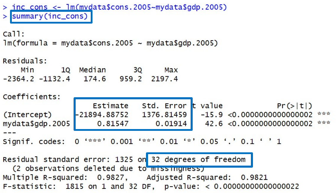
| Term | Estimate | Std. error | t value |
|---|---|---|---|
| Intercept | -21894.88752 | 1376.81459 | -15.9 |
| GDP | 0.81547 | 0.01914 | 42.6 |
Residual standard error 1325 on 32 degrees of freedom; ; on 1 and 32 DF.
Check slide 50 against the data descriptionThe slide says 34 yearly observations (1975 to 2008) and the output prints "2 observations deleted due to missingness", yet reports 32 degrees of freedom (which equals only if ). The slides use the printed 32 df, and so do I.
CIs for using , (slide values, rounded):
| Level | Critical value | Interval |
|---|---|---|
| 90% | 1.694 | |
| 95% | 2.036 | |
| 99% | 2.738 |
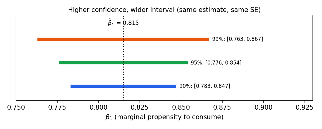
Same estimate, same standard error: only the multiplier grows with confidence. The limiting 100% interval is .
Example 2: housing prices
Model: , 88 US apartments (price in dollars, bdrms = number of bedrooms, sqrft = area in square feet).
Interpretation (log-log and log-level, see Lec_13-Exam Review):
- : percentage change in price for a 1% increase in area, all else equal (an elasticity).
- : percentage change in price from one more bedroom, all else equal (as a proportion; 0.038 is about 3.8%).
- : log price when and no bedrooms (area of 1 square foot).
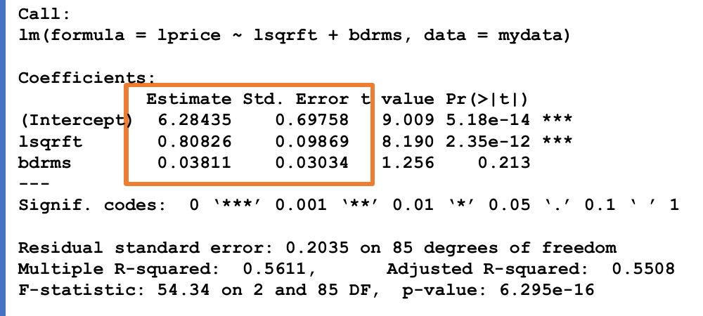
| Term | Estimate | Std. error | t value | p |
|---|---|---|---|---|
| Intercept | 6.28435 | 0.69758 | 9.009 | 5.18e-14 |
| lsqrft | 0.80826 | 0.09869 | 8.190 | 2.35e-12 |
| bdrms | 0.03811 | 0.03034 | 1.256 | 0.213 |
Residual standard error 0.2035 on 85 df; , adjusted ; on 2 and 85 DF.
The slides use a critical value of 2 (the large-sample approximation to ):
| Coefficient | 95% CI (slide, critical value 2) |
|---|---|
| bedrooms | |
| square footage |
Reading the intervalsThe bedrooms interval contains 0, so at 95% we cannot rule out that an extra bedroom has no effect on price once area is controlled for (consistent with ). The area interval is far from 0. This link between "CI contains 0" and hypothesis tests is exactly what the next lecture develops; the slides only say the machinery "will be used to calculate confidence intervals and to conduct simple hypothesis tests".
Summary of the t results
| Result | Formula |
|---|---|
| Intercept | |
| Slope | |
| CI |
4. Change of units
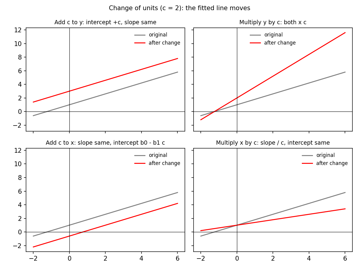
Question: if we add a constant to, or multiply, and/or , what happens to the estimated parameters? Start from and let . Tildes denote the new regression's parameters. The method on every slide: rewrite the new equation in the form , then match intercepts and slopes with the original.
Adding a constant to
New equation , i.e. . Matching: and .
The line shifts up by ; the slope is unchanged.
Multiplying by
New equation , i.e. . Matching gives
Both the intercept and the slope are scaled by .
Adding a constant to
New equation . Matching: and .
The slope is unchanged; the intercept adjusts (the line shifts horizontally). The slide leaves the summary boxes for this case blank; the answer is this derivation (slide 70).
Multiplying by
New equation . Matching: and .
Summary table
| Change | Slope | Intercept |
|---|---|---|
Common mistakes
- Rescaling scales the slope up by ; rescaling scales it down by (a regressor in thousands of shekels gets a slope 1000 times larger than one in shekels).
- Adding a constant to changes only the intercept (not the slope), and by , not .
- The slides state that the change of variables affects the estimators and their standard errors in the same way as above: a coefficient scaled by has its standard error scaled by , so t statistics and CIs transform consistently (a CI in new units is the old CI rescaled). The slides assert this without proof.
Check with unitsIf is in dollars and in metres, is dollars per metre. Switch to centimetres () and the slope must be 100 times smaller to describe the same relationship: .
Summary
- Estimate by ; the divisor reflects degrees of freedom lost to estimated parameters.
- The standard error is the square root of the estimated variance of .
- With A5 (normal errors) is normal; standardising with the estimated variance gives , with fatter tails than the normal.
- A CI is . It widens with a larger standard error or a higher confidence level; it is always centred on .
- Practical reading: take estimate and standard error from
summary(), get from the table orqt. - Change of units rules: shifts the intercept; scales both; changes only the intercept (); divides the slope by .
Related notes
- Intro Econometrics (course hub)
- Lec_08-Goodness of Fit & Multicollinearity
- Lec_13-Exam Review (covers CIs, t tests and units across the whole course)
- Assign_01-Interpreting OLS Output & the Birthweight-Smoking Regression, Assign_03-Change of Variables, Regression Through the Origin & the Housing Model
- Previous: Lec_04-OLS Estimator Properties — unbiasedness, variance and the classical assumptions
- Next: Lec_06-Hypothesis Tests & p-values — t tests and p-values