
OLS Estimator Properties
- #intro-econometrics
- #OLS
- #sampling-distribution
- #unbiasedness
- #efficiency
- #gauss-markov
- #classical-assumptions
- #homoskedasticity
- #variance-of-estimator
OLS Estimator Properties
Part of: Intro Econometrics | Key concepts: Sampling Distribution, Unbiasedness, Efficiency, Classical Assumptions, Zero Conditional Mean, Homoskedasticity, Gauss-Markov Theorem, Variance of the OLS Estimator
Where this lecture sits
Recap from the previous lecture
- OLS Estimation picks to minimise the sum of squared Residuals .
- That gives two first order conditions (FOCs): (residuals sum to zero) and (residuals are uncorrelated with in the sample).
- The theoretical model (unobserved errors , true line) is not the same thing as the fitted model (residuals , estimated line). The two lines differ, so in any given sample.
The question for today: are OLS estimates the best we can get? The lecture answers in four steps:
- What is a sampling distribution, and what do unbiasedness, minimum variance and efficiency mean?
- Which assumptions (A1 and A2) make OLS unbiased, with a proof.
- Which extra assumptions (A3 and A4) give a formula for the variance of OLS?
- The Gauss-Markov Theorem: under A0 to A4, OLS is the best linear unbiased estimator (BLUE).
1. The sampling distribution
Why estimates vary
and are functions of the sample . Draw a different sample from the same population and you get slightly different estimates. The collection of all these estimates is the estimator's sampling distribution: it shows how much the estimate moves purely because of which sample you happened to draw.
Review: the sample meanThe first estimator you met is for the population mean . Take a sample of size , compute , repeat times: the histogram of the averages is the sampling distribution of . (If is normal with unknown variance, standardised has a Student's t distribution.)
The simulation in the lecture
The slides run a demonstration in R (the lecturer stresses you do not need to know the code):
| Step | What is done |
|---|---|
| 1 | Generate a "population" of 1 million observations: , with . True values: , . |
| 2 | Take 1,000 samples, each of size . |
| 3 | In each sample, run the regression and save . |
| 4 | Plot histograms of the 1,000 estimates of each. |
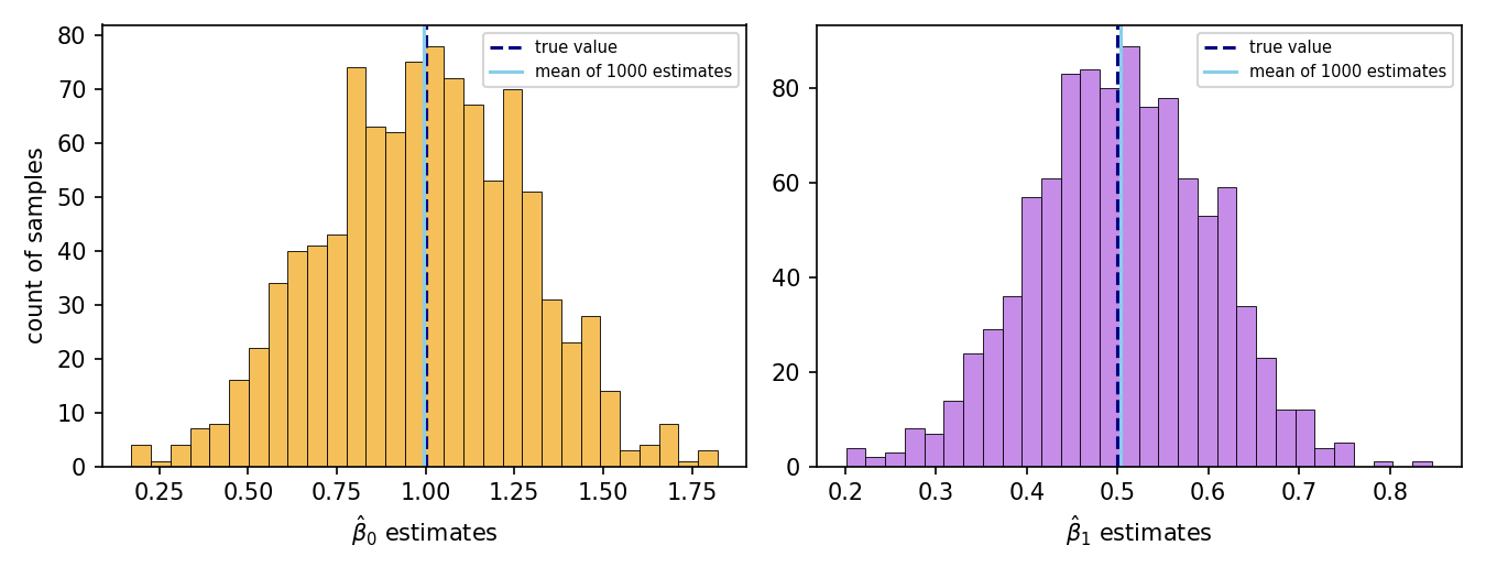
The histograms are bell-shaped and centred on the true values: the average of the estimates is about 1 for the intercept and about 0.5 for the slope, even though any single estimate can be well off.
Reconstructed from the slidesThe figure below is my re-run of the same data generating process with a fresh random seed (the slide's own histograms are an image of the lecturer's run). It reproduces the same picture: means of the 1,000 estimates are about 0.995 and 0.504, with spread (standard deviation) about 0.28 for the intercept and 0.10 for the slope.
2. Properties of an estimator
An estimator is a recipe (function) that turns any sample into an estimate. Many recipes can target the same parameter. For the population mean the slides list:
- Sample average:
- Silly estimator 1:
- Silly estimator 2:
To compare recipes we look at two moments of the sampling distribution of :
| Moment | Property it measures |
|---|---|
| Expected value | Unbiasedness |
| Variance | Minimum variance |
| Both together | Efficiency |
Unbiasedness
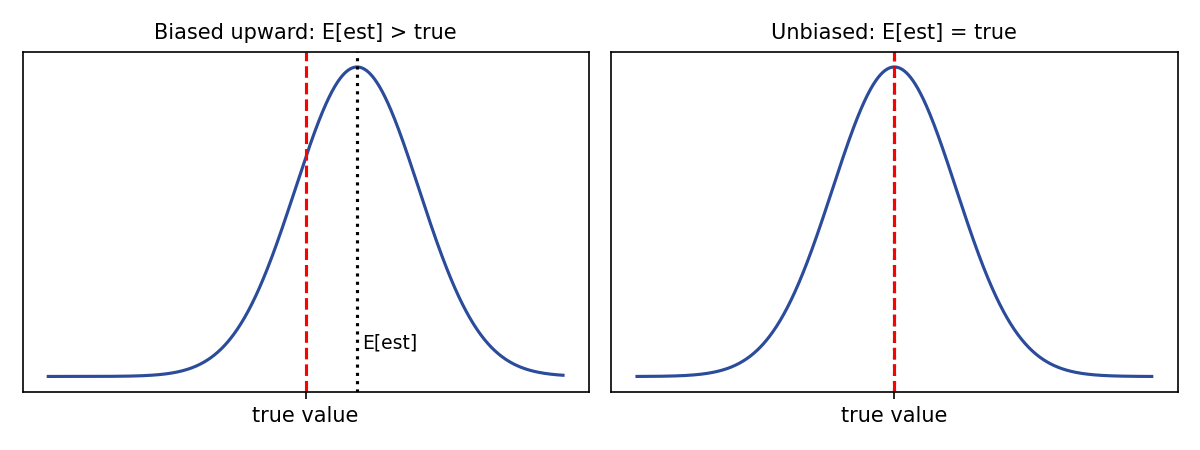
is an unbiased estimator of if the mean of its sampling distribution equals the true parameter:
- If the estimator is biased upwards; if it is biased downwards.
- Any single estimate can be wrong; unbiased means right on average (the average mistake is zero).
Minimum variance and efficiency
- An estimator has minimum variance if its sampling variance is less than or equal to that of any other estimator in the comparison class. Low variance means estimates from different samples cluster tightly, so a single estimate is likely to be close to its own mean.
- Efficiency combines both: an efficient estimator has the minimum variance among all unbiased estimators. Unbiasedness is a necessary condition for efficiency. Between two unbiased estimators, the efficient one is the one with the lower variance.
The slides pose these questions without answering themWhy is minimum variance important? Because you only ever see one sample. With a high-variance estimator your one estimate could be far from the truth even though it is right on average. Bias versus minimum variance? The slides leave this open. It is a genuine trade-off (a slightly biased estimator with much lower variance can land closer to the truth), but this course restricts attention to unbiased estimators and picks the lowest variance among them.
Activity 4, part 1: four estimators
True value . Legend of the four sampling distributions: Red (mean 0, variance 0.2), Green (mean 0, variance 1), Blue (mean 0, variance 2), Purple (mean , variance 0.5).
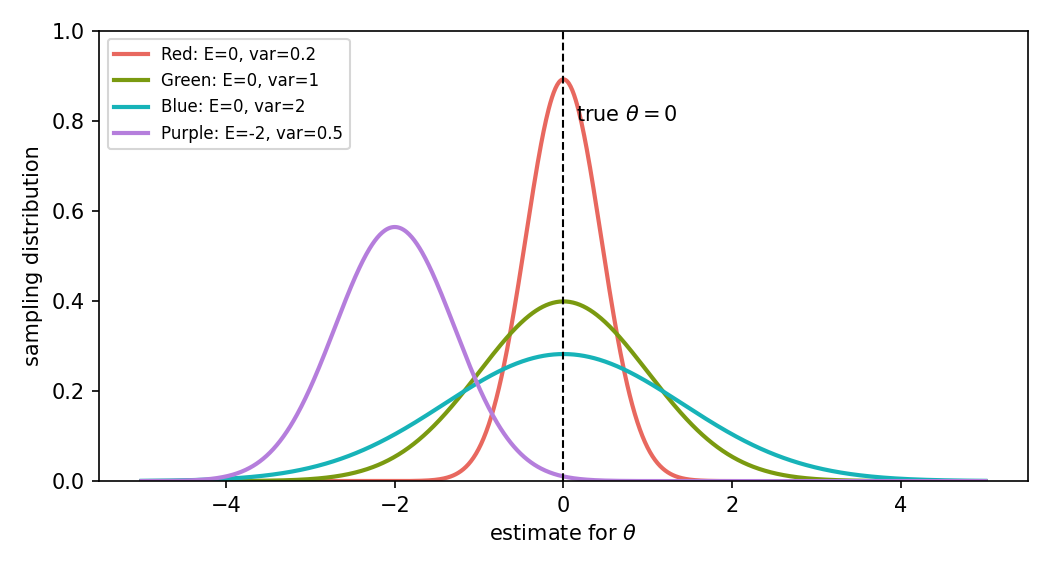
Reconstructed from the slidesThe slide asks the questions; the answers below are mine, read off the legend (I redrew the plot from the legend values).
| Question | Answer | Why |
|---|---|---|
| a) Unbiased? | Red, Green, Blue | Their means equal the true . |
| b) Biased? | Purple | Mean is (biased downwards). |
| c) Lowest variance? | Red (0.2) | Narrowest curve. Note Purple (0.5) has lower variance than Green and Blue but is biased. |
| d) Better of Green or Blue? | Green | Both are unbiased; Green has variance 1 versus 2, so Green is the more efficient of the two. |
Among the four, Red is the efficient estimator: unbiased with the smallest variance. Purple shows that low variance alone is not enough.
3. When is OLS unbiased? Assumptions A1 and A2
OLS is not automatically efficient: it needs assumptions about the data. All of them concern the random error , because:
- is a random variable whose realised values are unobserved.
- We cannot make assumptions about and (they are observed) or about (they are fixed numbers, not random).
Check the assumptions before you estimateIf the assumptions are reasonable for your sample you can use OLS. If not, a different method is needed.
Assumption 1 (A1): errors have mean zero
- The average error in the population is zero. This is weak: any non-zero average can be absorbed into the intercept, so the true line passes through the middle of the cloud of observations.
- Careful: it is about the unobserved errors , not the residuals , and the sample average is not necessarily 0.
Assumption 2 (A2): zero conditional mean
- The explanatory variable carries no information about the error. For every regressor : .
- This is the most important and most demanding assumption. See Zero Conditional Mean.
Wage regression and TOEFL (slide 34)Model: . The error bundles intelligence, luck, motivation and so on. Let (a TOEFL exam score) be one component of . A2 says : knowing someone has 10 versus 15 years of schooling tells you nothing about their expected English score. If in reality , then and A2 fails. In an English-speaking country A2 might hold; elsewhere we should worry.
- A2 cannot be tested directly, because the components of are unobserved. There are methods for when we suspect it fails (later in the course). This is the same idea as Omitted Variable Bias.
A1 and A2 imply zero covariance
Proposition: if A1 and A2 hold, then .
The first term is zero because A2 implies (marked with a star on the slide), the second because by A1.
Reconstructed from the slidesThe slide writes the first step as . The standard justification is the law of iterated expectations: .
Example: A1 holds but A2 fails (slide 37)
True model with equally likely, and
The errors average to zero overall (so A1 holds) but and (so A2 fails). All the observations at sit above the true line and all at sit below it, so OLS tilts the wrong way.
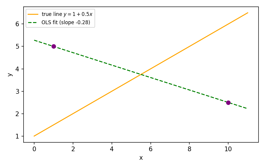
Reconstructed from the slidesThe slide only shows the two clusters and the true line. The OLS line in my figure is computed from the two group means, and : slope versus the true . This is the bias that a violated A2 causes.
Activity 4, part 2: link to the FOCs
Reconstructed from the slidesa) The two OLS first order conditions are and . b) They are the sample versions of A1 and A2: mirrors , and mirrors (which follows from A2). OLS forces these to hold in the sample by construction. A1 and A2 are the claim that they also hold for the true errors in the population.
Why assumptions are needed: the big picture (slide 39)
The population data generating function produces unobserved errors and observed regressors . The theoretical model then produces . From the observed we minimise squared residuals to get .
| Derived from the observed sample (FOCs) | Assumptions on the population |
|---|---|
| A1: | |
| A2: |
The FOCs let us compute the estimates; A1 and A2 guarantee they are unbiased relative to the true parameters. Two more assumptions are needed for efficiency.
4. Proof of unbiasedness
We work conditional on the sample of regressors and show .
Slope
Step 1: distance between estimate and parameter. Substitute into the OLS formula:
Split into three terms. The term vanishes because deviations from the average sum to zero, . The term cancels with the denominator to leave :
Step 2: take the conditional expectation. The denominator is non-random given , so it leaves the expectation; the expectation of a sum is the sum of expectations:
By A2, , and by A1 this is , so the numerator is :
ResultUnder A1 and A2, the OLS slope estimator is unbiased. The proof only used these two assumptions.
Intercept
Start from . Substituting and averaging:
Now plug in the slope result and collect the coefficient on each :
Activity 4, part 3 (the exercise left blank on slide 46): conditional on , the bracket is a constant, so
because by A2 and A1. Hence .
Reconstructed from the slidesSlide 46 (the answer to part 3) is an empty box in the deck, so the last step above is my completion, following the slope proof.
5. Efficiency: A3, A4 and the Gauss-Markov Theorem
Unbiasedness only needed A1 and A2. For minimum variance we add two more assumptions.
Assumption 3 (A3): no serial correlation
Errors of different observations are independent of one another. See Serial Correlation.
- Cross-sectional data: weak and unrestrictive, it follows directly from an iid random sample.
- Time series data: problematic (errors are often correlated over time). The lecturer says time series methods come next semester.
Assumption 4 (A4): homoskedasticity
The variance of the error is the same for every value of the explanatory variables. When it varies with , the model is heteroskedastic: . See Homoskedasticity and Heteroskedasticity.
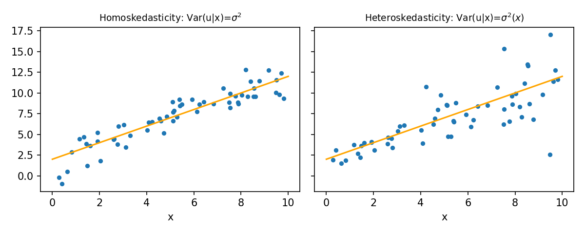
Income and consumption (slide 55)Low-income households have a small spread of consumption around the line (small error variance); high-income households have a large spread (large error variance). So A4 usually does not hold in this income-consumption context. The lecturer says heteroskedasticity-robust estimation comes at the end of the semester; see Lec_12-Heteroskedasticity.
Reconstructed from the slidesThe scatterplots on slides 54 and 55 are schematic. The pair of panels above is my own simulated illustration of the same idea, not data from the deck.
The classical assumptions together
| Label | Assumption | How reasonable? (slide 56) |
|---|---|---|
| A0 | The relationship is linear in the parameters | (the model itself) |
| A1 | Almost always true | |
| A2 | Most restrictive; often fails in economic models, but there are remedies | |
| A3 | Depends on how the data were sampled; can be fixed | |
| A4 | Usually holds; if not, it can be fixed |
Variance of the slope estimator
Conditional on , start from (the denominator equals ).
Each step and the assumption it uses:
- Adding a constant () does not change the variance, so it drops out.
- The denominator is a constant, so it is squared and pulled outside the variance.
- A3 (errors uncorrelated): the variance of the sum is the sum of the variances.
- A2: the 's are fixed given , so comes out of the variance squared.
- A4: for every , so it factors out of the sum.
- Cancel the common term in numerator and denominator.
Variance of the intercept estimator
Stated without proof (the slide calls it "a nice exercise to try practising at home"; all four assumptions are used):
What drives the variance of OLS
The variance formulas have the error variance on top and the sample variation in , , below:
| Driver | Effect on estimator variance |
|---|---|
| Larger variance of the random error | Larger (noisier data, less precise estimates) |
| Larger spread of the in the sample | Smaller (more variation in identifies the slope better) |
| Larger sample size | Smaller (more terms in ; also in the intercept formula) |
More on how this variance changes with correlated regressors in Lec_08-Goodness of Fit & Multicollinearity. See Variance of the OLS Estimator.
The Gauss-Markov Theorem
Gauss-Markov TheoremIf the relationship is linear (A0) and A1 to A4 hold, then the OLS estimators have the minimum sampling variance of any unbiased estimator. In other words, OLS is the Best Linear Unbiased Estimator (BLUE).
- The lecture proves unbiasedness (section 4) and derives the variance (section 5), but not the final step that this variance is the minimum. That proof needs linear algebra and is in the course textbook's appendix.
- The slides prove it for the single-regressor case; the theorem holds for multiple regression as well.
- See Gauss-Markov Theorem.
How to remember what each assumption buys
- A0 + A1 + A2 OLS is unbiased (slope and intercept).
- A3 + A4 (on top) the variance has the clean form and OLS has the smallest variance among unbiased linear estimators: BLUE.
- If A4 fails, OLS stays unbiased but is no longer efficient and the usual variance formula is wrong (fix: robust standard errors, see Lec_12-Heteroskedasticity).
6. Looking ahead (slide 62)
The next lectures use these results for inference:
- Estimate and plug it into to get the standard error of .
- Use the standard error to build a Confidence Interval in which the true probably lies.
- Use that to test hypotheses, for example whether is statistically different from 0 (t-test).
Quick revision checklist
- State the definition of an unbiased estimator and of an efficient estimator.
- Explain why a single estimate can be wrong even if the estimator is unbiased.
- Write A0 to A4 and say which one drives unbiasedness (A1, A2) and which drive the variance formula (A3, A4).
- Reproduce the slope unbiasedness proof: substitute, use , take , apply A2 then A1.
- Write and say how , the spread of and affect it.
- Give an example where A2 fails (omitted TOEFL-like variable correlated with schooling).
- Explain what Gauss-Markov says and what it does not say (it needs A1 to A4).
Related notesCourse-wide revision of unbiasedness, the classical assumptions and testing: Lec_13-Exam Review. Applied practice with OLS output: Assign_01-Interpreting OLS Output & the Birthweight-Smoking Regression.
- Previous: Lec_03-Nonlinear Models with OLS — logs and nonlinear functional forms
- Next: Lec_05-Confidence Intervals & Change of Units — confidence intervals and change of units