
Multiple Hypothesis Tests
- #intro-econometrics
- #f-test
- #joint-hypothesis-test
- #restricted-model
- #hypothesis-testing
- #OLS
- #returns-to-scale
Multiple Hypothesis Tests
Part of: Intro Econometrics | Key concepts: F-test, Joint Hypothesis Test, Restricted Model, Unrestricted Model, Residual Sum of Squares, t-test, Returns to Scale
Where this lecture sits
Quick recap (week 3 material)
- The multivariate model is ; each is the effect of holding all other variables fixed.
- OLS Estimation minimises ; the partial derivatives give first-order conditions , .
- In R:
summary(lm(y ~ x1 + x2 + x3 + x4, mydata)).- A single coefficient is tested with a t-test or a Confidence Interval.
New this lecture: how to test several restrictions at once with an F-test, and how to build the restricted model for any null hypothesis. The later lectures reuse this machinery: Lec_08-Goodness of Fit & Multicollinearity (joint significance when t-stats are all small) and Lec_11-Interaction Terms (Chow-type joint tests on dummies and interactions). The whole course is summarised in Lec_13-Exam Review; practice is in Assign_04-Omitted Variables, F-tests & Multicollinearity (Birthweight & Soda Prices).
Title slide vs contentThe title slide also lists "regression through the origin" and "change of units". The 37 slides cover only multiple hypothesis tests, so those two topics are not in this note.
1. Warm-up: reading one coefficient (Activity 7, part 1)
Model on 540 US workers (2002):
| Variable | Estimate | Std. error | t | p |
|---|---|---|---|---|
| (Intercept) | 1.385217 | 0.4218969 | 3.28 | 0.001 |
| s | 0.0981245 | 0.0108345 | 9.06 | 0.000 |
| exp | 0.0402309 | 0.0056855 | 7.08 | 0.000 |
| IQ_test | 0.0112204 | 0.0029018 | 3.87 | 0.000 |
| age | -0.0336168 | 0.0101734 | -3.30 | 0.001 |
| hours | 0.0041505 | 0.0024687 | 1.68 | 0.093 |
Residual SE 0.49889 on 534 df; , adjusted ; on 5 and 534 df.
Effect of age: , so one more year of age lowers wage by about 3.36% (log-level model, so multiply by 100). It is significant at 10%, 5% and 1% (), so we reject . The 95% interval is
Why this matters for what followsA t-test answers "is this one coefficient zero?". It cannot answer "are and both irrelevant?" or "does ?". Those are joint hypotheses, so we need the F-test.
2. Joint hypotheses
Take and test that and both have no effect:
The alternative is "everything else"is true if at least one restriction fails: , or . It is not "both are non-zero".
An F-test compares two models:
| Unrestricted model (UR) | Restricted model (R) | |
|---|---|---|
| What it is | the original model we care about | the original model with the null imposed |
| Example | ||
| Parameters | free | forced by |
See Unrestricted Model and Restricted Model.
3. Building the restricted model
Substitute the null into the model, then simplify. Always start from .
| Null hypothesis | Restricted model | What is new |
|---|---|---|
| and | variables dropped | |
| , , | (no intercept) | intercept and variables dropped |
| and | new variable | |
| and | new explanatory variable | |
| and | new dependent variable |
Rule of thumb (slide 20)
- If a restriction fixes a coefficient to a non-zero constant (), the restricted model has a new outcome variable ().
- If a restriction ties coefficients together (), the restricted model has a new explanatory variable (combine and ).
- If it sets a coefficient to zero, just drop the variable.
Activity 7, part 2.
- or or .
- Unrestricted: the full four-regressor model.
- Restricted: .
- Rearranged: .
- New variables: dependent variable and explanatory variable .
4. The F-statistic
Residual sum of squares
See Residual Sum of Squares (written SSR in some notes; same thing).
Key fact:
Why dropping variables can never lower the RSS (slide 22)OLS picks the coefficients that minimise RSS. The unrestricted model has all the freedom of the restricted one plus more: it could choose and copy the restricted estimates exactly, giving the same RSS. Since it can always do at least that well, it never does worse. So unless the unrestricted estimates happen to satisfy the null exactly, in which case they are equal.
Idea of the test: if the null is (nearly) true, imposing it barely raises the RSS, so the gap is small. If the null is false, forcing it costs a lot of fit and the gap is large.
The statistic
| Symbol | Meaning |
|---|---|
| RSS of the unrestricted model | |
| RSS of the restricted model | |
| number of restrictions in the null | |
| degrees of freedom of the unrestricted model | |
| number of observations | |
| number of first-order conditions (estimated parameters) in the unrestricted model, i.e. |
The denominator isis the unbiased estimator of the error variance in the unrestricted model (the textbook remark on slide 34). So is "extra RSS per restriction" measured in units of the noise level.
Computing
: the difference in degrees of freedom, which equals the number of parameters removed. With observations and (UR has df):
| Null | Restricted model | ||
|---|---|---|---|
Shortcutis just the number of equals signs you are testing (count independent restrictions). Use the df difference to double check.
Decision rule
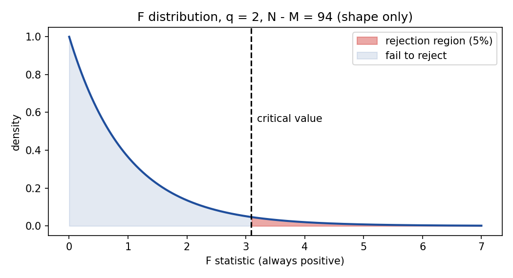
- The distribution takes only positive values, so the rejection region is a single right tail: reject if .
- If , we fail to reject the null.
- Critical values come from the table in the formula sheet (slide 26 shows the 5% table: columns are , rows are ; the "infinity" row for gives 2.37) or from R.
5. Relation between the F-test and the t-test
When there is a single restriction () the two tests are the same test:
Slide 27 illustrates with an R regression of consumption on GDP: and the ANOVA F value is .
Only forFor two or more restrictions there is no t-test equivalent. A joint test can reject even when each individual t-test fails to reject, and vice versa. This is exactly the situation with highly correlated regressors (see Lec_08-Goodness of Fit & Multicollinearity).
6. Worked example: electricity production cost (Activity 7, part 3)
Setup
Cost is a Cobb-Douglas function (Cobb-Douglas Function) of output and the prices of fuel , labour and capital :
Data: 99 monthly observations (cost in millions of dollars, output in billions of kWh). Taking logs makes it linear ( becomes the intercept):
OLS output (unrestricted model)
| Variable | Estimate | Std. error | t | p |
|---|---|---|---|---|
| (Intercept) | -8.548757 | 1.394584 | -6.13 | 0.000 |
| ln_y | 0.824102 | 0.013085 | 62.98 | 0.000 |
| ln_pk | 0.2028625 | 0.1445721 | 1.40 | 0.164 |
| ln_pl | 0.1778888 | 0.142561 | 1.25 | 0.215 |
| ln_pf | 0.6932505 | 0.0807074 | 8.59 | 0.000 |
Residual SE 0.21197 on 94 df; , adjusted ; on 4 and 94 df.
InterpretationThe coefficient on is an Elasticity: a 1% rise in output raises cost by about 0.8%, less than 1%. This means Returns to Scale are increasing: doubling output less than doubles cost, which is the signature of a natural monopoly (the slide's own conclusion).
Test of constant returns to scale
Constant returns means cost grows one-for-one with output. The null fixes a coefficient to a non-zero constant, so (by the rule in section 3) the restricted model has a new dependent variable:
From R (anova(...)["Residuals",2]): and . Here , , , so , and .
Since we reject constant returns to scale.
Same answer from the t-test
, so reject. And , matching exactly, as the relation predicts.
Typo on the slidesSlide 33 writes "13.433^2 = 180.71". The t-statistic on the same slide is 13.443 and , so 13.433 is a typo.
Summary
- A t-test handles one restriction; an F-test handles restrictions at once (Joint Hypothesis Test).
- Write , (any restriction fails), the unrestricted model, and the restricted model (impose and simplify).
- Restricted-model recipe: zero restrictions drop variables; creates a new dependent variable ; creates a new explanatory variable.
- always, because OLS minimises RSS and the unrestricted model has more freedom.
- ; ; reject if (right tail only).
- For : and the two tests agree.
- Electricity example: (elasticity below 1, increasing returns); , so constant returns to scale is rejected.
Related notes
- Intro Econometrics (subject hub)
- Lec_08-Goodness of Fit & Multicollinearity, Lec_11-Interaction Terms, Lec_12-Heteroskedasticity
- Lec_13-Exam Review (whole-course review, includes t and F tests)
- Assign_04-Omitted Variables, F-tests & Multicollinearity (Birthweight & Soda Prices), Assign_04-Solutions (Answer Key)
- Assign_02-Functional Form & the Money-Supply Log-Log Model (log-log elasticities)
- Previous: Lec_06-Hypothesis Tests & p-values — t tests and p-values
- Next: Lec_08-Goodness of Fit & Multicollinearity — goodness of fit and multicollinearity