
Statistics Review & OLS Estimation
- #intro-econometrics
- #statistics-review
- #expected-value
- #variance
- #covariance
- #correlation
- #iid
- #estimator
- #OLS
- #residuals
- #population-regression-function
- #sample-regression-function
Statistics Review & OLS Estimation
Part of: Intro Econometrics | Key concepts: Expected Value, Variance, Covariance, Correlation, Statistical Independence, IID Sample, Estimator, OLS Estimation, Population Regression Function, Sample Regression Function, Residual
Two decks, one noteLecture 2 had two slide decks. Part 1 (17 slides) is a statistics refresher: the tools needed to say anything about an estimator. Part 2 (47 slides) introduces the simple regression model and derives the OLS formulas from scratch. Later topics (properties of OLS, tests, confidence intervals) are summarised in Lec_13-Exam Review; practice on this material is in Assign_00-R Data Cleaning & Statistics Review and Assign_01-Interpreting OLS Output & the Birthweight-Smoking Regression.
Part 1 — Statistics review
Random and non-random variables
- A random variable has a probability distribution over possible values; what we see are observations drawn from that distribution.
- A non-random variable takes one value. Convention: capital letters are random; lower-case are non-random. A non-random may change between observations but is still non-random (it is a fixed, known number for each , e.g. a weight).
Distribution and density
- Distribution function: .
- Density function: when the derivative exists.
- Properties: and .
The slide also writesThat holds for a probability (mass), but a density of a continuous variable can exceed 1 (e.g. a narrow normal). Only and total area are guaranteed. Treat the upper bound as a slide simplification.
The Normal distribution
has two parameters, mean and variance :
- The standard normal has mean 0, standard deviation 1.
- Standardise: .
- Theorem: a linear transformation of a normal random variable is also normal. (This is what later lets , a linear combination of normal errors, be normal.)
Expected value (mean)
A location measure: . Linearity is the property used constantly:
With non-random weights and random :
Expectation passes through sums and constantsof a sum is the sum of s always, with no conditions. Variance is different (below).
Variance and standard deviation
It measures how far values of typically are from the mean. Standard deviation (same units as ).
| Property | Statement |
|---|---|
| Constant | |
| Scaling | |
| Shift and scale | (adding a constant changes nothing) |
| Sum | |
| Difference | |
| Three terms |
Variance of a sum is NOT the sum of variancesUnlike expectation, in general. They are equal only when the covariance is zero. This is why independence (zero covariance) of observations matters so much for the variance of and of .
Covariance
- : the variables move together (positive relationship); : they move oppositely.
- Property 1: the covariance of a random variable with a constant is zero, . Proof: , or .
- Property 2: for constants ,
Correlation
A covariance rescaled to be unit-free and bounded:
- : perfect positive linear relation; : perfect negative; : no linear relation.
- Uncorrelated means , which is the same thing as zero covariance.
Statistical independence
and are independent if their joint density is the product of the marginals, . Equivalently (for all functions of them, not just the identity). Plugging into the covariance formula, independence gives .
Zero covariance does NOT imply independenceIndependence is the stronger property. The converse fails, as the coin example shows.
Worked example: uncorrelated but dependent
Flip a coin. if Head, if Tail. For : if Tail, ; if Head, flip again, for head and for tail.
- and .
- .
So : uncorrelated. But , so depends on (when , is forced to 0).
| If... | Then |
|---|---|
| independent | covariance zero and uncorrelated |
| covariance zero (or uncorrelated) | may or may not be independent |
IID samples
An iid (independent, identically distributed) random sample is draws from the same distribution , each independent of the others. Practically:
- every observation has the same mean:
- every observation has the same variance:
- any two have zero covariance: for
Estimators
An estimator of a parameter is a function of the random sample, , which gives a number for each realised sample. Example: the sample average estimates the population mean.
Class average vs university averageThe average height in this class is an estimate of the average height at the university. It is generally not identical to the parameter. If the class is a random sample, the sample average is the "best" estimator: minimum variance and unbiased.
The sample analogues of each population moment (the "best" estimators):
| Parameter (population, unobserved) | Estimator (sample) |
|---|---|
Why ?Dividing by (not ) makes the sample variance unbiased: the deviations are measured from , not the true , which uses up one degree of freedom. The slides state the formula without deriving it.
Part 2 — OLS estimation
The income-consumption question
We want the effect of income on consumption, and (assuming a causal reading, which the lecture flags with "is this reasonable?") the slope is the marginal propensity to consume. Even with data on the whole population, households with the same income do not consume the same amount, so points will not lie on one line.
Population model, error, and sample
Assume a linear relationship in the population (the "theoretical model"):
- is the theoretical line (impossible to observe, since we cannot gather the whole population).
- is the random error: the vertical gap between observation and the theoretical line. It captures everything that affects consumption other than income and varies across individuals.
In practice we have an iid sample (the slide shows 10 households with income in thousands and consumption):
| Household | 1 | 2 | 3 | 4 | 5 | 6 | 7 | 8 | 9 | 10 |
|---|---|---|---|---|---|---|---|---|---|---|
| Income | 50 | 45 | 70 | 100 | 37 | 75 | 60 | 100 | 37 | 95 |
| Consumption | 40 | 37 | 50 | 60 | 37 | 54 | 58 | 85 | 20 | 93 |
The scatter shows a positive relationship.
PRF vs SRF
Two different lines, one from the population and one from the sample:
| Population Regression Function (PRF) | Sample Regression Function (SRF) | |
|---|---|---|
| Model | ||
| Parameters | : true, unobserved | : estimates from OLS |
| Error term | : random error, unobserved | : residual, computed |
| Fitted line | theoretical line |
The SRF is an estimator of the PRF. We want it unbiased with minimum variance, but the two lines will not coincide exactly (a different sample gives a different SRF). The whole course is about using a sample to draw conclusions about the population: how to compute , why they are "best" under certain assumptions (you must understand the proof for the exam, not write it), and what the estimates say about the unobserved s.
Terminology
- : dependent / outcome / endogenous variable. : independent / explanatory / exogenous variable.
- : intercept of the theoretical model. : slope, the change in for a one-unit change in holding the error fixed (all else fixed).
- : anything affecting other than ; its sign puts the observation above or below the line.
- : the predicted value, a point on the SRF.
- Residual: : observed minus predicted. It is an estimate of the error .
Activity 2 (part 1): computing residualsSuppose and .
- Household 10 (income 95, consumption 93): .
- Household 9 (income 37, consumption 20): .
(The slide writes the intermediate step as "", a sign slip; the answers 2.25 and -16.45 are right.) Positive residual: point above the line.
Reconstructed from the slides: Activity 2 (part 2), counting solutionsThe slides pose three questions on four data points; the answer slides are mostly diagrams, so the reasoning below is mine.
- Know : each residual is then pinned down, so one value per observation.
- Know two residuals: two points on a line (both observed points shifted by known amounts) determine the line uniquely, so one pair.
- Know only : the slope is fixed but the intercept is free, so infinitely many combinations (a family of parallel lines).
A line is determined by slope and intercept, or a point and a slope, or two points.
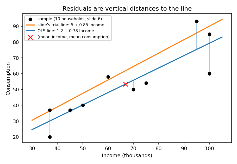 Theory diagram built from the slide's 10-household sample: the orange line is the slide's trial line, the blue line is the OLS line I computed (, , which the lecture does not state). Thin blue segments are the OLS residuals. The OLS line passes through the sample means (red cross).
Choosing the line: why squares
Two decisions define an estimator: (1) how to measure the distance of each point from the line, and (2) how to aggregate across observations.
- Sum of residuals : fails, because points below the line have negative residuals, so the minimiser is a line far from the data.
- Absolute value of the sum : fails, because many different lines give exactly zero (positives and negatives cancel), so it does not identify one line. The slides show two different lines each with zero residual sum.
- Sum of squared residuals : no cancellation, and it penalises large misses heavily. This is OLS:
- Ordinary: the simplest method to calculate
- Least: because we minimise
- Squares: because we use the squared residuals
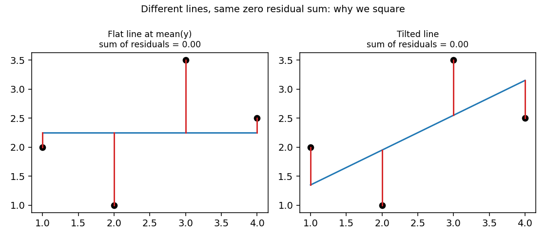 Theory diagram (my toy data, not the slide's): two quite different lines, both with residuals summing to exactly zero, so "sum of residuals" cannot pick a line.
Other loss functions existInstead of squaring we could use the absolute value of each residual, etc. Different functions yield different estimators; OLS is just the standard one.
Deriving the OLS estimators
The data are fixed; we search over . To minimise: take the partial derivative with respect to each, set both to zero, solve.
Partial derivative w.r.t. (chain rule on each squared term, inner derivative ):
Partial derivative w.r.t. (inner derivative ):
The first order conditions (FOCs)
Two equations, two unknowns.
What the FOCs say(1) residuals sum to zero (so they average zero); (2) residuals are uncorrelated with in the sample. These two facts reappear in every later lecture.
Solving FOC (1): the intercept
Two consequences: this gives the intercept as a function of the slope and the data, and the regression line passes through the sample means, .
Solving FOC (2): the slope
Substitute into :
The slide then notes (and refers to HW0 / the stats review) that numerator and denominator can be rewritten with , because and :
Reading the slope formulaThe slope is the sample covariance of and divided by the sample variance of . Positive covariance means a positive slope. (The factors cancel in the ratio.)
OLS summary
| Estimator | Formula |
|---|---|
| Intercept | |
| Slope | |
| Fitted value | |
| Residual |
Statistical vs economic modelling
If we flip the model to , the same method gives
Both are valid statistical estimators, but only one has economic meaning. The computer cannot tell which variable causes which: that is the economist's job. (Recall Lecture 1: correlation is not causation.)
Example: US consumption vs GDP
Data: real personal consumption expenditure (Cons) and real GDP, both in billions of 2012 dollars, 75 quarterly observations 2002 to 2020. Model: .
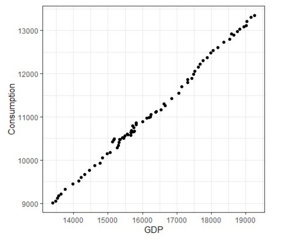 Real data (cropped from slide 43): consumption against GDP is almost perfectly linear.
By hand in R (from cov() and var() output on the slide):
Or with lm(Consumption ~ GDP, data = FRED.data), which reports:
| Coefficient | Estimate |
|---|---|
| (Intercept) | |
| GDP |
Fitted model: .
Interpretation (Activity 2 part 4)
- Slope: one extra billion (2012) dollars of GDP goes with 742 million more consumption; equivalently, 74.2 cents of each dollar of income go to consumption, or 74.2% of income is consumed (the marginal propensity to consume).
- Intercept: when GDP is zero, predicted consumption is billion. Not interesting: GDP of zero is far outside the data (an extrapolation), and negative consumption is meaningless.
The flipped regression
lm(GDP ~ Consumption) gives intercept and slope : the "computer doesn't know which is the correct model".
Reconstructed check (not on the slides)matches the flipped slope ( from the
var(Consumption)output). Note : the flipped slope is not the reciprocal of the original, since (here about 0.997, so close).
Comparison: PRF vs SRF vs the two regressions
| Idea | Population | Sample |
|---|---|---|
| Line | ||
| Gap from line | error (unobserved) | residual (computed) |
| Known? | never | always, from data |
Summary
- Stats toolkit: is linear; needs covariance terms; in ; independent uncorrelated but not the reverse.
- iid sample: same mean and variance, zero pairwise covariance. Estimators are functions of the sample; moments are estimated by sample averages ( for variance and covariance).
- Model: PRF (unobserved); SRF (estimated).
- OLS minimises (not , which cancels). FOCs: and .
- Solution: , ; the line passes through .
- Regression is statistical; which variable is is an economic choice.
Related notes
- Intro Econometrics (hub)
- Lec_13-Exam Review: whole-course review covering OLS properties, tests and confidence intervals
- Lec_08-Goodness of Fit & Multicollinearity: uses the FOCs and the SSR/TSS decomposition built here
- Assign_00-R Data Cleaning & Statistics Review and Assign_01-Interpreting OLS Output & the Birthweight-Smoking Regression
- Concepts: Expected Value, Variance, Covariance, Correlation, Estimator, OLS Estimation, Residual
- Previous: Lec_01-Introduction & Causal Inference — causal effect, confounders, the regression model
- Next: Lec_03-Nonlinear Models with OLS — logs and nonlinear functional forms