
Introduction & Causal Inference
- #intro-econometrics
- #causal-inference
- #correlation-vs-causation
- #population-regression-function
- #confounding
- #randomised-experiment
Introduction & Causal Inference
Part of: Intro Econometrics | Key concepts: Causal Effect, Population Regression Function, Error Term, Correlation vs Causation, Confounding Factor, Randomised Experiment
Course logistics (brief)
The first third of the deck is course admin. The parts worth keeping for the exam:
- Assessment: exam is 100 points, in person, open notes (20 pages one-sided), closed internet, with an extra formula sheet. You must score 60 on the exam (before the HW bonus) to pass. Five homeworks give up to 2 bonus points each (10 total), only if submitted on time; no late homework for any reason.
- Homework: groups of up to 3, may write up individually or submit as a group (one copy for the group). Part A is theory and interpreting R output, Part B is R coding.
- Exam style: theory, interpreting R output, and handwritten R "pseudo-code".
- AI is not permitted this semester: the goal is to build econometric thinking first. Next semester the course teaches AI tools alongside estimation.
- Reading: Wooldridge, Introductory Econometrics: A Modern Approach (3rd edition or later), chapters 1 to 8 plus Appendices A, B and C; Heiss, Using R for Introductory Econometrics (2nd edition) chapters 1 to 8.
Study pattern from the slidesStay up to date weekly, start homework early, work alone first until stuck, then use office hours, recitation and peers.
Course schedule (13 weeks)
| Week | Lecture topic |
|---|---|
| 1 | Introduction, causal inference, statistics and maths review |
| 2 | Ordinary Least Squares (OLS) estimation |
| 3 | Nonlinear relations in OLS; briefly the multivariate regression |
| 4 | Estimator properties and the classical assumptions behind them |
| 5 | The standard error and the confidence interval |
| 6 | Hypothesis tests using OLS estimates |
| 7 | The multivariate model, changing units, regression through the origin |
| 8 | Goodness of fit and multicollinearity (Lec_08-Goodness of Fit & Multicollinearity) |
| 9 | Quadratic terms, model misspecification |
| 10 | Dummy variables (Lec_10-Dummy Variables) |
| 11 | Interaction terms, Chow-Fisher tests (Lec_11-Interaction Terms) |
| 12 | Heteroskedasticity-robust standard errors, WLS (Lec_12-Heteroskedasticity) |
| 13 | Review (Lec_13-Exam Review) |
Lectures are Tuesday afternoons with a Sunday TA recitation (R coding). The homework schedule is in the Intro Econometrics hub.
1. What is econometrics?
Econometrics takes the theories from other economics courses and checks them against data:
- estimate the model the theory proposes;
- judge its performance: does the theory play out in reality, and which of two competing models fits the real world better?
- use the results to test hypotheses, which in turn are used to set policy.
The central goal is to estimate the effect of on . The slides list pairs from many fields:
| Field | (outcome) | (cause) |
|---|---|---|
| Economics | Growth, unemployment, wage | Taxes, minimum wage, education |
| Social science | Grades, crime rate, house prices | Class size or teacher wage, police presence, capital gains tax |
| Beyond social science | Health, recovery, global temperature | Exercise, cancer treatment, CO2 emissions |
2. The model: a causal relation between and
In its simplest form the claim " affects " is written as a straight line:
- is the intercept: the value of when .
- is the slope: the change in for a one-unit change in . This is the causal relation between and .
The slides show the sign and size of carries the economics:
| Question | Slope | Reading |
|---|---|---|
| Does education affect wage? | More years of education, higher wage | |
| Does class size affect learning? | Yes, somewhat (grades fall with class size) | |
| Does class size affect grades? | , steeper | Yes, considerably |
| Does skills training affect earnings? | Nope: flat line, no effect | |
| Does training affect wage? | Yes |
In-class activity (slide 30)Think of a case where should lower (class size and grades), and one where could push either way depending on the underlying process (for instance, a policy that both raises demand and raises costs).
The general model
Real data never sit exactly on a line, so we add a noise term:
The same equation goes by several names: the true model, the theoretical model, or the population regression function. The slides motivate it by the potential-outcomes framework (not taught here; see Angrist and Pischke, Mostly Harmless Econometrics, and Cunningham, Causal Inference: The Mixtape), in which is the average treatment effect.
| Symbol | Name |
|---|---|
| outcome variable (dependent variable) | |
| explanatory variable (independent variable) | |
| noise or error: everything other than that affects | |
| intercept (a parameter) | |
| slope (a parameter) |
Wage modelHere holds skill, luck, motivation and everything else that moves wages. is the effect of one more year of education on wage.
3. The basic problem of econometrics
and are unknown population parameters. The slides make two points:
- We will never know their value with certainty; all we can do is estimate them from observed data.
- Often we cannot estimate them well. The goal of the course is to learn when and how good estimation is possible.
In-class activity (slide 38)Think of a causal relationship where collecting data is hard or impossible, and one where data are easy to collect but the causal effect is not very useful to measure.
Data versus the true line
With data we observe pairs for each observation (for example years of education with wage, with , and so on in the slide's table). Each observation satisfies the data generating process
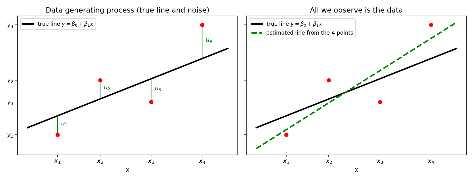
Reconstructed from the slidesThe slide draws four generic points with the true line, noise terms (vertical gaps), and then a flatter estimated line through the same dots. The figure above is my redraw of that picture with four illustrative points; the numbers are made up for the diagram and are not course data.
Key consequences:
- are unknown, so each is unknown too, and so is the true regression line.
- All we observe is the data. An estimated line fitted to a sample will generally differ from the true line (the lectures that follow build OLS to make that estimate as good as possible).
4. Why is hard to learn: the "what if" problem
is a counterfactual quantity: what would happen to if changed, everything else held fixed?
- We can never know what you would earn had you not studied here.
- We cannot know whether a cancer patient would have lived longer had she taken the new drug.
- We cannot observe the same child in a class of 20 and a class of 30 at once.
Each unit in the data has experienced one value of and no other. So the individual counterfactual problem is impossible to solve; we use data on many units and estimate the average effect.
5. Correlation is not causation
Worked example: wages and education (1976 US census, CPS)
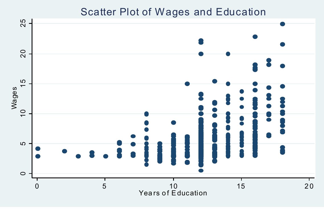
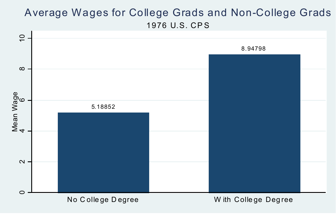
What the data showMean wage is 5.19 for people without a college degree and 8.95 for those with one (1976 US CPS, Current Population Survey). The scatter shows wages rising with years of education, with a lot of spread at each level.
So statistically there is a positive correlation between wage and education. But does that say anything about ? No. People with more education may also have wealthier parents or a more stable family background; those factors raise wages even if the causal effect of education were 0. Even when a causal effect is plausible, it is hard to measure.
More examples from the slides
| Example | Correlation observed | Why it fails as a causal claim |
|---|---|---|
| Running and health | Runners are healthier | Runners may also eat better, smoke less (confounding factors) |
| Dog at home and children's blood pressure (Israeli study reported in Haaretz) | Children with a dog had lower blood pressure under mild stress | Children with dogs may exercise more (walking the dog) or have calmer parents |
| GDP per capita and COVID-19 deaths (Our World in Data, 19 April 2020) | Richer countries show more confirmed deaths per million | Reporting and testing capacity, age structure and travel links may drive both |
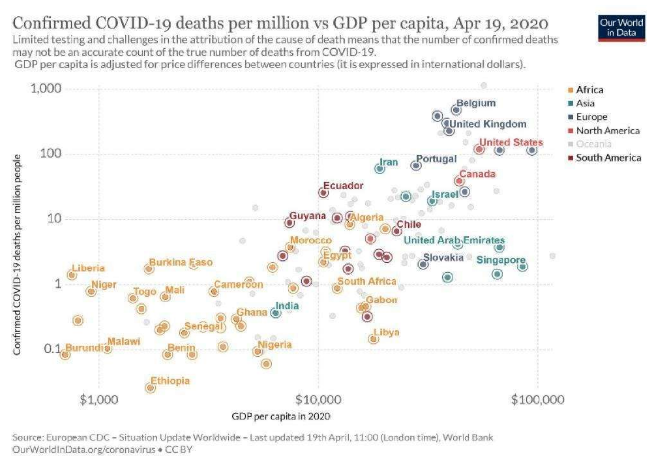
Reconstructed from the slidesThe COVID slide gives only the title question and the chart. The listed confounders for it are my reading of the slide's own chart caveat (limited testing, attribution of deaths), not a claim made on the slide.
Correlation versus causation formally
Correlation is a purely statistical concept:
We want the causal effect, not correlation, and correlation alone says nothing about causality. Everything is possible:
- no correlation but a causal relationship exists;
- strong correlation but no causal link;
- positive correlation but a negative causal effect.
In-class activity (slide 59)Give an example with a causal effect but no observed correlation, and one with positive correlation but negative causal effect (the police and crime example below is the second type).
Common mistakeReading a regression slope as "the effect of on " without asking what else differs between high- and low- units.
6. Example: police and crime
Theory says (more police, less crime). Yet the data (Crime2.dat) show the opposite:
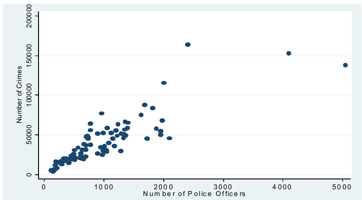
The correlation between number of police officers and number of crimes is 0.86. The slide's explanation: big cities have both more police and more crime, so we are looking at two variables with no causal link between them that are both tied to a third variable, city size (a confounder).
Controlling for city population by looking at per capita figures gives a very different picture:
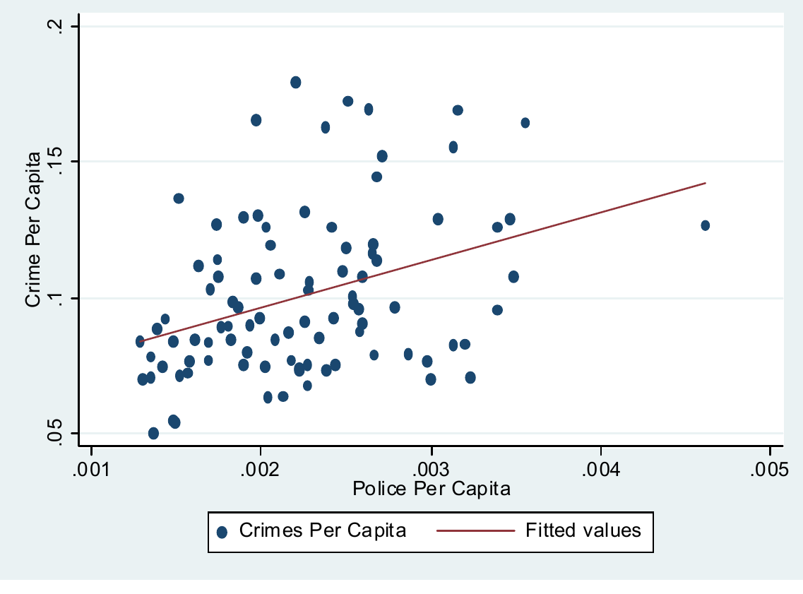
The correlation drops to 0.37 (still positive, as the fitted line shows). The slides then cite Levitt (AER 1997), who shows the causal effect is negative () once this problem is handled properly. Conclusion: here correlation is not causation.
IntuitionPutting variables on a per-person basis removes the pure size effect, but the correlation is still positive: controlling for one confounder does not make the regression causal. The rest of the course is about what controlling for factors does and does not buy you.
7. How can we estimate causality? Randomisation
Consider .
- We can estimate the drug's causal effect only if the experiment is random.
- If the drug goes only to the sickest patients we cannot learn its causal effect (the same logic: if more police are sent to neighbourhoods with more crime).
- The crucial question is always: is the assignment of random or not?
Random assignment makes unrelated to everything in , so differences in can be attributed to .
Why reality is not a random experiment
Data are mostly observed, not collected in an experiment. We cannot randomise which university you attend, class size, or teacher pay. Economists run more experiments now (for example job training and wages), but experiments are often unethical, infeasible or expensive.
In-class activity (slide 66)Vaccination uptake and infection rates: what makes the vaccine's effect hard to estimate? (People who choose to vaccinate may differ in age, behaviour and health, and vaccination spreads in waves with the epidemic itself. These are my notes, not the slide's.)
Conclusion from the lecture
- The main obstacle to empirical research is that reality is not a random experiment.
- In these cases we cannot prove a causal effect, only assume it exists. Before computing we must be convinced that plausibly explains .
- Next semester focuses on causal inference; this semester focuses on the mechanics of estimation (OLS and its properties).
Summary
- Econometrics tests economic theories on data and estimates the effect of on through the model (population regression function), where collects all other factors.
- are unknown; the best we can do is estimate them from a sample, so the estimated line differs from the true one.
- is a counterfactual: each unit is seen at one value of only.
- Correlation is not causation: confounders (family background, city size) can create or hide a relationship, even reversing its sign (police and crime).
- Random assignment is the clean way to learn a causal effect, but economics mostly has observational data, so this course focuses on estimation mechanics and flags causal assumptions.
Related notes
- Intro Econometrics (hub) and _Intro Econometrics Concepts
- Lec_13-Exam Review covers the whole course, including the OLS topics that follow this lecture
- Assign_01-Interpreting OLS Output & the Birthweight-Smoking Regression (Assign_01-Solutions (Answer Key)) uses a regression and asks for a causal reading
- Lec_08-Goodness of Fit & Multicollinearity, Lec_10-Dummy Variables
- Next: Lec_02-Statistics Review & OLS Estimation — statistics review and the OLS first-order conditions