
Nonlinear Models with OLS
Nonlinear Models with OLS
Part of: Intro Econometrics | Key concepts: Functional Form, Log-Level Model, Log-Log Model, Elasticity, Marginal Effect, Simple Linear Regression, Residuals, Prediction, Linear in Parameters, Rate of Change
Where this fitsWeeks 1 and 2 set up causality and the mechanics of OLS. This lecture's one big idea: OLS can fit curved relationships, as long as the model is linear in the parameters. Take logs, and a nonlinear story becomes a linear regression. The second half previews the multiple regression model. The full-course view of this material is in Lec_13-Exam Review; applied practice is in Assign_02-Functional Form & the Money-Supply Log-Log Model and Assign_03-Change of Variables, Regression Through the Origin & the Housing Model (Assign_02-Solutions (Answer Key), Assign_03-Solutions (Answer Key)).
0. Recap of last week (slides 3 to 5, 9 to 10)
- PRF (population): . 's and are unobserved; observed. is everything else affecting .
- SRF (sample): ; prediction .
- OLS minimises . First-order conditions: and .
- Estimators: and
Activity 3 part 1 (slides 9 to 10)Given , , :
Only the covariance and the variance of matter; is a distractor.
1. Running example: the wage model
Goal: estimate the effect of education on wage, . Data: Israel, 2014 household survey (slides 6 to 8). Summary statistics on the slide: hourly wage has median 40.218, mean 53.661, max 976.115 (6,228 missing); years of schooling has median 13, mean 13.82, max 61, n = 16,499. The wage distribution is right-skewed.
Level-level fit and why it fails (slides 13 to 18)
Level-level model: , so . This is the marginal effect and it is constant: the model assumes a linear relation.
Estimated line:
| Years of schooling | Predicted hourly wage |
|---|---|
| 15 | |
| 16 | |
| 0 | (negative wage!) |
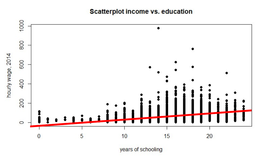 Real data from slide 15: the straight line sits below most points at high schooling and goes below zero at low schooling.
Problems the slide raises:
- Every extra year adds a flat 5.9 NIS, but the data suggest the gain grows with education.
- The line predicts a negative wage at zero schooling, which is impossible.
Slide 17 also recalls how to get and in R: fitted(myreg) and resid(myreg). Each residual is the observed wage minus the line's prediction (the highlighted point is an observation above the line, residual about 42.6).
The fix: an exponential relation (slides 19 to 21)
Wages are never negative and rise convexly with schooling, so model
Take natural logs of both sides, using :
Key ideaThis is linear in its parameters , so OLS applies directly. The relation between and is nonlinear, but the regression is linear in the transformed variable. This is the log-level model. As a bonus, predicted wage is always positive, so the negative-wage problem disappears.
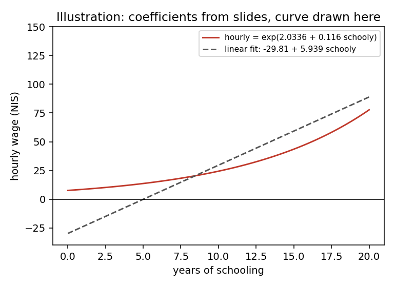 Illustration drawn here from the slide coefficients (not slide data): the exponential curve stays positive and bends upward, the straight line does not.
2. The log-level model
Interpretation: the slope is the rate of change, i.e. the proportional change in per one-unit change in . A one-unit rise in raises by about percent. Here it measures the returns to a year of education.
In R the default base of log() is (natural log). Activity 3 part 2 asks for the code to estimate it; with a data frame mydata the answer is along the lines of lm(log(hourly) ~ schooly, data = mydata) (the slides use a pre-computed ln_hourly column in the plot code).
Slide 24: estimated
Schooling (slide, rounded) 12 3.4 29.96 13 3.5 33.12 14 3.7 40.45 The NIS gap between rows changes, but the percent change is constant at 11.6%: one more year of school adds 11.6% to wage.
Rounding on the slideThe slide rounds the log to one decimal before exponentiating. Unrounded, , so the 12-year prediction is , not 29.96 (and 13 years gives about 34.5, 14 years about 38.8). Also, in logs is an approximation: the exact percent change is . For the exam, follow the rule " percent".
Fit: the log-level model fits the data better than level-level (slide 25).
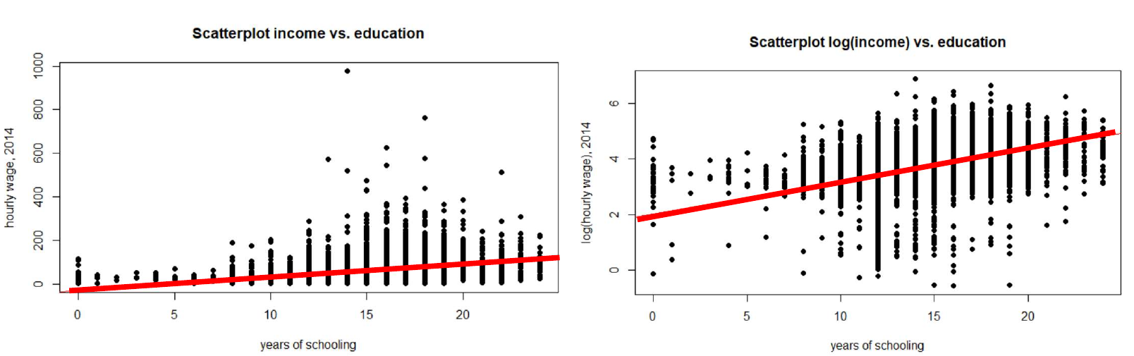 Real data from slide 25. Left: wage in levels with the OLS line, a poor fit. Right: log wage against schooling, where the line tracks the cloud.
The intercept (slide 26): with zero schooling the predicted wage is , which is always positive. The slide also notes the model assumes a constant rate of change, while the marginal effect in NIS () increases with education.
3. The log-log model and elasticity
Both sides in logs. The slope is the elasticity of with respect to :
The log-log model assumes a constant elasticity, which is why it is the standard model for demand: .
Demand curves (slide 29)Linear demand has elasticity that changes along the curve: at the top (at ), at the midpoint, at the bottom. Constant-elasticity demand (a hyperbola-type curve) has the same elasticity everywhere; the slide labels it 1.5, i.e. .
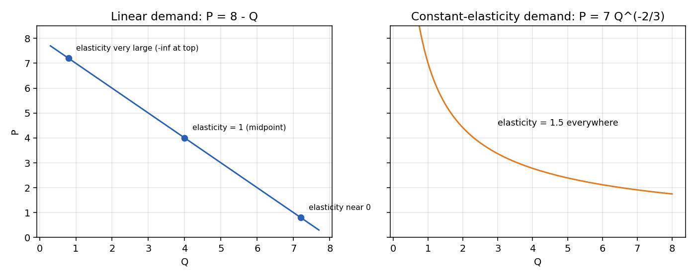 Theory diagram redrawn from slide 29.
Reconstructed from the slidesWhy gives elasticity 1.5: invert to , so . The log-log slope is , i.e. . The slide only labels the number.
Wage example (slides 30 to 31)
gives, on the slide, intercept and slope .
- is the wage elasticity of education: a 1% rise in schooling raises wage by about 1.5%. Since , wage is "elastic" with respect to education.
- But the slide stresses that this model does not fit the data well.
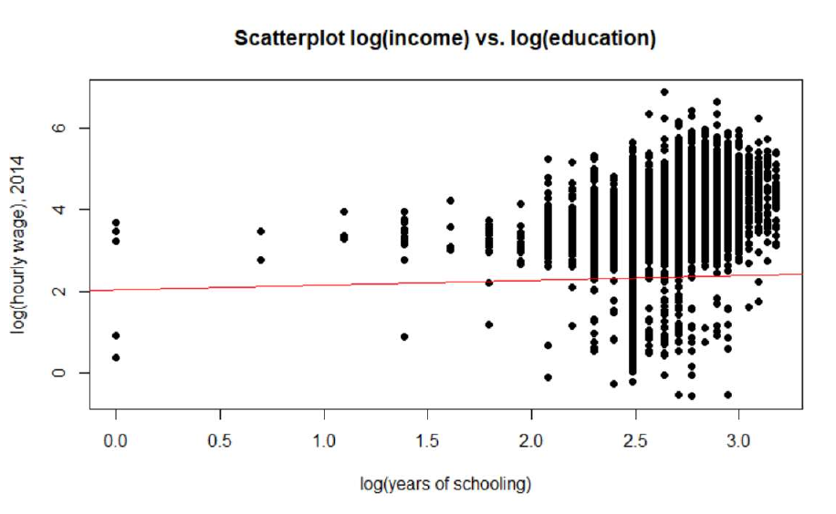 Real data from slide 31: log wage against log schooling. The red line on the slide is very flat, which does not look like a slope of 1.5; the printed coefficients and the plotted line may come from different samples. Treat the "poor fit" message as the point.
4. Which model should you use? (slides 33 to 34)
Technically any of the models can be estimated. Choose by:
- Fit to the data (compare the plots), and
- Theory and past research: wage models conventionally use log-level, demand models log-log.
Selection depends on the variables, not on which economic moment you want to compute (slide 43).
| Model | Equation | Slope reads as | Statement |
|---|---|---|---|
| Level-level | Marginal effect | unit units | |
| Log-level | Rate of change | unit percent | |
| Log-log | Elasticity | percent percent (no ) | |
| Level-log | Units per percent | a percent change in changes by a number of units (about ) |
Rule of thumbThe variable that carries the log is measured in percentages. The level-log "" step is not spelled out on the slide beyond "units of per percentage change of "; the full table is in Lec_13-Exam Review.
Limits of OLS (slides 35 to 36)
- OLS needs the model to be linear in the parameters after transforming variables. Log-log is fine: minimise , giving and . The same FOCs hold: and .
- If no transformation makes the model linear in its parameters (the slide's example is a form with the parameter inside a nonlinear expression), OLS fails; you need NLLS or GMM instead.
5. Economic moments for every model (slides 37 to 42)
Three ways to describe the effect of on :
Each model's slope equals one of these; the others follow by multiplying by , , or .
| Moment | Level-level | Log-level | Log-log |
|---|---|---|---|
| Slope is | |||
| Marginal effect | (constant) | ||
| Rate of change | (constant) | ||
| Elasticity | (constant) |
Activity 3 part 3 (slides 41 to 42)Log-log: from , multiply by to get marginal effect ; multiply by to get rate of change ; elasticity .
- In the level-level model the marginal effect is constant but the rate of change and elasticity vary with and . The elasticity is usually reported at the sample means: (slide 39).
- In each model exactly one moment is constant, and that moment is the slope itself.
6. A first look at multiple regression (slides 44 to 52)
Usually one regressor is not enough. With explanatory variables:
- : the effect on when all are fixed at zero (the constant).
- : the effect of on holding all other variables fixed.
- OLS minimises ; the partial derivatives give first-order conditions: and for each .
- Adding genuinely explanatory variables increases the explained part () and reduces the unexplained part ().
- In R:
summary(lm(y ~ x1 + x2 + x3 + x4, mydata)).
Wage regression example (slides 50 to 52)
US data from 2002, subsample of 540 observations. Model (slide): ; the R call on the slide also includes hours.
| Variable | Estimate | Std. Error | t | p |
|---|---|---|---|---|
| (Intercept) | 1.385217 | 0.4218969 | 3.28 | 0.001 |
| s (schooling) | 0.0981245 | 0.0108345 | 9.06 | 0.000 |
| exp | 0.0402309 | 0.0056855 | 7.08 | 0.000 |
| IQ_test | 0.0112204 | 0.0029018 | 3.87 | 0.000 |
| age | -0.0336168 | 0.0101734 | -3.30 | 0.001 |
| hours | 0.0041505 | 0.0024687 | 1.68 | 0.093 |
Residual standard error 0.49889 on 534 df; Multiple , Adjusted ; F-statistic 46.02 on 5 and 534 df, p-value .
Activity 3 part 4: interpretation (not worked on the slides)The dependent variable is a log, so each slope is a rate of change, holding the other regressors fixed.
- Schooling: one more year raises wage by about 9.8% (significant, ).
- Experience: one more year raises wage by about 4.0%.
- IQ test: one more point raises wage by about 1.1%.
- Age: one more year lowers wage by about 3.4% holding experience, schooling and the rest fixed. This is a "holding experience fixed" effect, not the raw age pattern.
- Hours: about 0.4% per extra hour, significant only at the 10% level ().
- Fit: the regressors explain about 30% of the variation in log wage.
7. Where the course goes next (slide 53)
- Lecture 1: causality and regression; Lecture 2: OLS notation and mechanics.
- Lecture 3 (today): nonlinear relations with OLS and a taste of multiple regression.
- Next: why OLS is the "best" estimator and under which assumptions (see Classical Assumptions), then confidence intervals (Confidence Interval) and hypothesis tests (Hypothesis Testing, p-value).
Summary
Takeaways
- OLS needs linearity in the parameters, not in the variables: logs let it fit curves.
- Level-level: slope = marginal effect (constant). Log-level: slope = rate of change ( for percent). Log-log: slope = elasticity (constant).
- Choose the model by fit and theory (wages: log-level; demand: log-log), not by the moment you want.
- Every model has all three moments; only the slope's own moment is constant.
- Log-level fixes the "negative wage" problem: .
- Multiple regression: each is a ceteris paribus effect; FOCs.
Related notes
- Previous: Lec_02-Statistics Review & OLS Estimation — statistics review and the OLS first-order conditions
- Next: Lec_04-OLS Estimator Properties — unbiasedness, variance and the classical assumptions
- Hub: Intro Econometrics