
Hypothesis Tests & p-values
- #intro-econometrics
- #hypothesis-testing
- #t-test
- #p-value
- #confidence-interval
- #one-sided-test
- #regression-through-origin
- #OLS
Hypothesis Tests & p-values
Part of: Intro Econometrics | Key concepts: Hypothesis Testing, Null Hypothesis, t-statistic, Critical Value, p-value, Confidence Interval, One-Sided Test, Regression Through the Origin
How this note connectsThe slides open with a recap of confidence intervals (Lecture 5 material). This note keeps that recap short and spends its length on the new material: t-tests, p-values, one-sided tests and regression through the origin. For the wider course (OLS, t and F tests, CIs) see Lec_13-Exam Review; for the regression-through-the-origin homework see Assign_03-Change of Variables, Regression Through the Origin & the Housing Model.
1. Recap: confidence intervals (from last time)
- A confidence interval satisfies . Here is the significance level (usually 5%) and the confidence level (usually 95%).
- With the symmetric t-distribution, the critical value solves , so . (Slides 3 to 11 build this with CDF shading: .)
- Under assumptions A1 to A5 (A5: normal errors ), is normal, and replacing the unknown with gives
- Hence the CI:
Activity 6 (part 1): 95% CI forhoursWage model
ln_earnings ~ s + exp + IQ_test + age + hours, , 534 df, . Forhours: estimate , s.e. .. The interval contains 0, which foreshadows
hoursnot being significant at 5%.
Estimation vs inference (slide 18):
| Stage | Question |
|---|---|
| Estimation | Given observations, which fits best? |
| Confidence interval | How likely is it that falls in a range around the true ? |
| Hypothesis test (today) | How probable is our sample if the true parameter were a specific value ? |
2. The two-sided t-test: four steps
A test never gives a certain "yes/no", only "with some probability no". Four steps:
- State and . In general against . Examples: slope equals 2; intercept equals 4; slope is zero ("does X affect Y?").
- Compute the t-statistic, taking and from the output and from the null:
- Pick the significance level (usually 5%; 10% and 1% are also checked) and find the critical value from the t-table.
- Decide.
- If : fail to reject . If is true this happens with probability .
- If : reject . If is true this (a false rejection) happens with probability , split as in each tail.
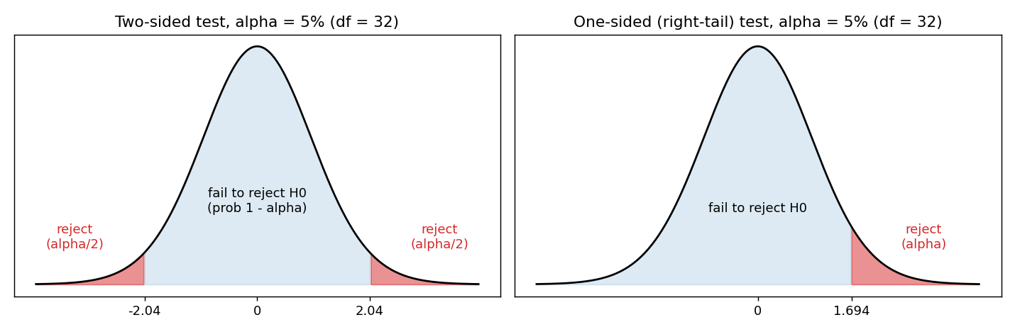 Theory diagram: rejection regions (red) and non-rejection region (blue) for a two-sided and a right-tail test at 5%, df = 32.
WordingSay "fail to reject", never "accept". Not rejecting only means the data are consistent with it; many other values of would also survive.
Example 1: income-consumption model
(Israeli data, 32 df). Output: , , , . Critical value .
| Question (all at ) | Decision | ||
|---|---|---|---|
| Does income affect consumption? | Reject: income matters | ||
| Do Israeli consumers not save? (MPC = 1) | Reject (slide left this blank; reconstructed) | ||
| Is the marginal propensity to consume 80%? | Fail to reject |
Example 2: housing prices
, 88 US apartments, 85 df. The slides use (nearest table row).
| Coefficient | Estimate | Std. Error | t value | Pr(>|t|) |
|---|---|---|---|---|
| (Intercept) | 6.28435 | 0.69758 | 9.009 | 5.18e-14 |
| lsqrft | 0.80826 | 0.09869 | 8.190 | 2.35e-12 |
| bdrms | 0.03811 | 0.03034 | 1.256 | 0.213 |
, adjusted , on 2 and 85 df.
| Question | Decision | ||
|---|---|---|---|
| Bedrooms do not affect price | Fail to reject | ||
| One more bedroom cuts price by 2% | slide: | Fail to reject | |
| One more bedroom raises price by 10% | slide: | Reject |
Rounding on slides 36 and 37With I get for and for . The slide values (1.933, -2.063) look like they use . The decisions are the same either way, and the is only just beyond .
3. Confidence intervals and two-sided tests are the same thing
We fail to reject iff , and rearranging (slide 32) gives
RuleIf is inside the CI, fail to reject at . If is outside, reject. This holds for two-sided tests only.
- Income-consumption: CI contains 0.8 (not rejected) but excludes 0 and 1 (rejected). Consistent with the three tests above.
- Housing: CI (slides use ) contains and but excludes . Again consistent.
4. Significance testing and p-values
Significance test
"Does have a significant effect on ?" is the special case vs , with
This is the t value column of R's summary(lm). Reject the variable is significant; fail to reject it has no significant effect on .
Careful (slides 42 and 43)The
t valuecolumn tests only . For any other null () you must compute yourself.
Activity 6 (parts 3): which variables are significant at 5%? (wage model, critical value 1.96)
Variable Estimate Std. Error t value Pr(>|t|) (Intercept) 1.385217 0.4218969 3.28 0.001 s 0.0981245 0.0108345 9.06 0.000 exp 0.0402309 0.0056855 7.08 0.000 IQ_test 0.0112204 0.0029018 3.87 0.000 age -0.0336168 0.0101734 -3.30 0.001 hours 0.0041505 0.0024687 1.68 0.093 , adj. , on 5 and 534 df. Every variable has except hours (): hours is not significant at 5%, but is at 10% ().
What a p-value is
The p-value is the minimum significance level at which we would reject for the observed t-statistic:
i.e. the probability, if were true, of a t-statistic at least as extreme as the one we observed. Half of sits in each tail. Small = strong evidence against .
Decision rule: reject at level iff .
| p-value | Reading | Decision |
|---|---|---|
| 0.5 | Half of samples would look this extreme under : weak evidence against | Do not reject |
| 0.072 | Only 7.2% of samples this extreme: some evidence | Not at 5%; would reject at 10% |
| 0.014 | Only 1.4%: evidence against | Reject at 5%, not at 1% |
- Income-consumption slope: , so we reject at any significance level above that.
- Housing
bdrms: . Wagehours: (the "." in the stars column marks significance at 10%).
Do not over-rely on p-valuesThe lecture stresses that p-values are widely misinterpreted and that leaning on them has contributed to reproducibility problems and p-hacking (trying specifications until ). A p-value is not the probability that is true.
5. One-sided tests
Same t-statistic ; only the rejection region changes: all of goes in one tail, so the critical value is (the 1-tailed row of the table, e.g. ), not .
| Left-tail test | Right-tail test | |
|---|---|---|
| Hypotheses | vs | vs |
| Reject when | ||
| Otherwise | fail to reject | fail to reject |
Table trick (slide 58)The t-table has a 1-tailed row and a 2-tailed row. For the same use the 1-tailed row for one-sided tests ( map to 1-tailed ), and the 2-tailed row for two-sided tests.
Example: marginal propensity to consume (df 32, )
| Decision | |||
|---|---|---|---|
| Fail to reject (needs ) | |||
| Reject (since ) | |||
| Fail to reject | |||
| Fail to reject |
Reconstructed from the slides: do the 0.8 results contradict each other?The slide asks this but gives no answer on the page. They do not contradict: failing to reject and failing to reject just says the data cannot separate from 0.8 in either direction ( is tiny relative to the critical value). Not rejecting is not accepting, so there is no inconsistency.
6. Summary of the testing procedure
- Write and .
- Compute the t-statistic.
- Get the critical value for the chosen (1-tailed or 2-tailed row, correct df).
- Compare and decide. Equivalent shortcut: reject iff (two-sided: iff the CI).
7. Regression through the origin
Sometimes theory says when , so the model has no intercept:
Both the theoretical and fitted lines pass through .
OLS estimator
Minimise . First-order condition:
| With intercept | Through origin | |
|---|---|---|
| Slope estimator | ||
| Equal when | only if | |
| Unbiased when | A1 to A4 hold (always, even if true ) | only if the true intercept is |
Which mistake is worse?
| Mistake | Consequence |
|---|---|
| Include an intercept although true | Minor: is just an estimate that should come out near 0; all estimates stay unbiased under A1 to A4. |
| Omit the intercept although true | Biased slope . |
Direction of the bias (slides 72 to 73): if the true , forcing the line through the origin makes it steeper, ; if , it makes it flatter, .
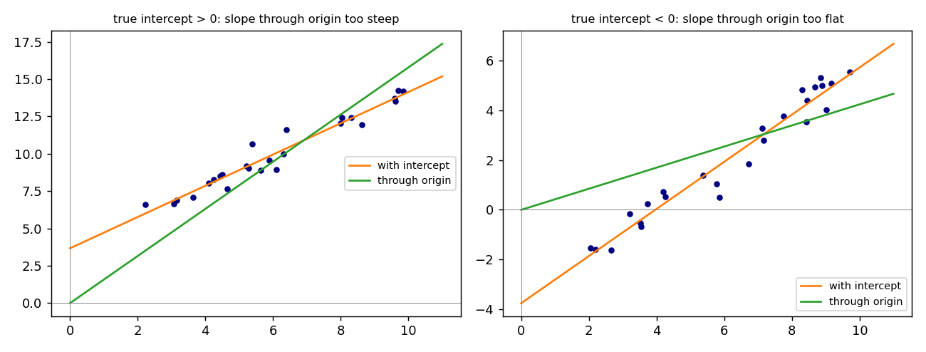 Theory diagram (simulated points, not course data): the green no-intercept line pivots about the origin and distorts the slope in the direction opposite to the sign of the true intercept.
Activity 7 (part 4): HW3 Part A Q3, income-consumption
A colleague argues a negative intercept is impossible (consumption cannot be negative) and so fits a no-intercept model. Output shown on slide 75:
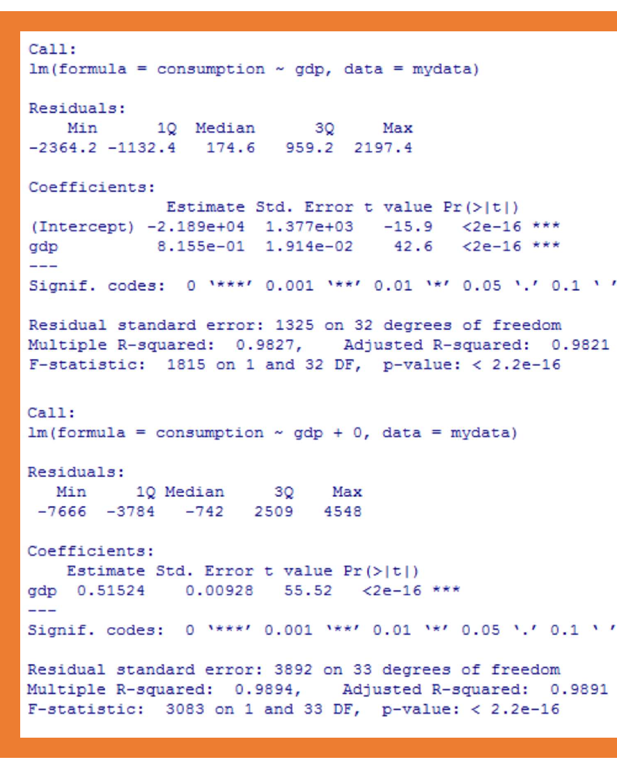 Real data: R output from slide 75, with-intercept model (top) and
gdp + 0 model (bottom).
| Model | Slope | s.e. | Intercept | Residual s.e. | |
|---|---|---|---|---|---|
| With intercept | 0.8155 | 0.01914 | -21890 (s.e. 1377, t = -15.9, p < 2e-16) | 1325 on 32 df | 0.9827 |
Through origin (gdp + 0) |
0.51524 | 0.00928 | none | 3892 on 33 df | 0.9894 |
Reconstructed from the slides: answers to (a) and (b)(a) Yes: the intercept has , , so it is significantly different from zero. (b) Use the model with the intercept: the true intercept is clearly not 0, so omitting it biases the slope, and indeed the slope drops from 0.8155 to 0.5152, consistent with the picture. The no-intercept model's higher printed (0.9894 vs 0.9827) is not comparable: is computed differently without an intercept, and its residual standard error (3892) is far worse than 1325.
The deck then shows "HW 4 Part A" (slide 76) with the sign pattern and ; the slide's regression output was not legible as text.
Should I include an intercept? (slide 77)
- Theory (though it does not always give an answer).
- Statistical tests: goodness of fit and a significance test on the intercept.
Summary
- A hypothesis test asks how plausible the sample is if . Four steps: hypotheses, , critical value, decision.
- Two-sided: reject iff ; equivalently iff lies outside the CI.
- The R
t valuecolumn tests only (significance). - The p-value is the smallest at which you reject; reject iff . Handle with care (p-hacking).
- One-sided tests use the same but a one-tail critical value ; "fail to reject" both sides is not a contradiction.
- Dropping the intercept when the true one is non-zero biases the slope; including a needless one is harmless.
Related notes
- Intro Econometrics (hub)
- Lec_13-Exam Review: whole-course review including t and F tests and CIs
- Lec_08-Goodness of Fit & Multicollinearity
- Assign_03-Change of Variables, Regression Through the Origin & the Housing Model and Assign_03-Solutions (Answer Key)
- F-test
- Previous: Lec_05-Confidence Intervals & Change of Units — confidence intervals and change of units
- Next: Lec_07-Multiple Hypothesis Tests — joint tests and the F-test