
Model Misspecification & Quadratics
- #intro-econometrics
- #model-misspecification
- #quadratic-model
- #omitted-variable-bias
- #irrelevant-variable
- #regression-through-the-origin
- #multicollinearity
- #confidence-interval
Model Misspecification & Quadratics
Part of: Intro Econometrics | Key concepts: Model Misspecification, Quadratic Model, Marginal Effect, Turning Point, Irrelevant Variable, Omitted Variable Bias, Regression Through the Origin, Multicollinearity, Confidence Interval
Where this lecture sits
The threadSo far the course assumed we knew which explanatory variables belong in the model. In practice we choose them ourselves, by trial and error. This lecture asks what goes wrong when we choose badly, and how a squared term lets one regressor have a curved effect. It builds on Lec_08-Goodness of Fit & Multicollinearity and is followed by Lec_10-Dummy Variables. The whole course is revised in Lec_13-Exam Review.
Recap from last week (slides 3 to 6), kept short:
- Perfect multicollinearity: an exact linear relation between regressors. Partial: a strong but inexact one.
- Detect partial collinearity indirectly via , the from regressing on all other regressors.
- High makes small and inflates the variance (see Variance of the OLS Estimator):
- Overall model significance uses the F-test of against the restricted model .
Today's agenda: quadratic terms, adding an irrelevant variable, omitting a relevant variable, then exam practice.
1. Model misspecification: the two errors
Two mistakes are possible when we pick regressors:
- Adding an irrelevant variable (one whose true coefficient is zero).
- Omitting a relevant variable (one that really affects ).
The lecture's verdict (section 5): the second is the more serious one.
2. Quadratic terms
Why add a square
When and have a parabolic relation, include both and in the regression. For :
| Sign of the squared coefficient | Shape | Effect of on |
|---|---|---|
| "happy" (U) | falls, then rises | |
| "sad" (inverted U) | rises, then falls |
Example: wages and experience (slides 11 to 16)
Hypothesis: wage rises with experience up to a point and then falls. Test it by adding expsq and checking whether its coefficient is significant.
| Term | Estimate | Std. error | t | p |
|---|---|---|---|---|
| (Intercept) | 6.792880 | 0.845662 | 8.033 | 3.22e-14 |
| educ | 0.077893 | 0.007134 | 10.919 | < 2e-16 |
| exp | 0.043415 | 0.009460 | 4.589 | 1.52e-05 |
| expsq | -0.000916 | 0.000355 | -2.582 | 0.0102 |
expsq is significant at 5%, so the relation is parabolic.
The marginal effect is no longer constant
Differentiating with respect to :
Activity 9 part 1: the slope at different experience levelsThe slides leave the answers blank; plugging in is mechanical.
Experience Reading 1 year 0.0416 about +4.2% wage per extra year 10 years 0.0251 about +2.5% 20 years 0.0068 about +0.7% 30 years -0.0115 about -1.2%: past the peak The slope shrinks as experience grows and turns negative after the peak.
The turning point
Set the derivative to zero (first-order condition) and solve:
General rule for : the Turning Point is at .
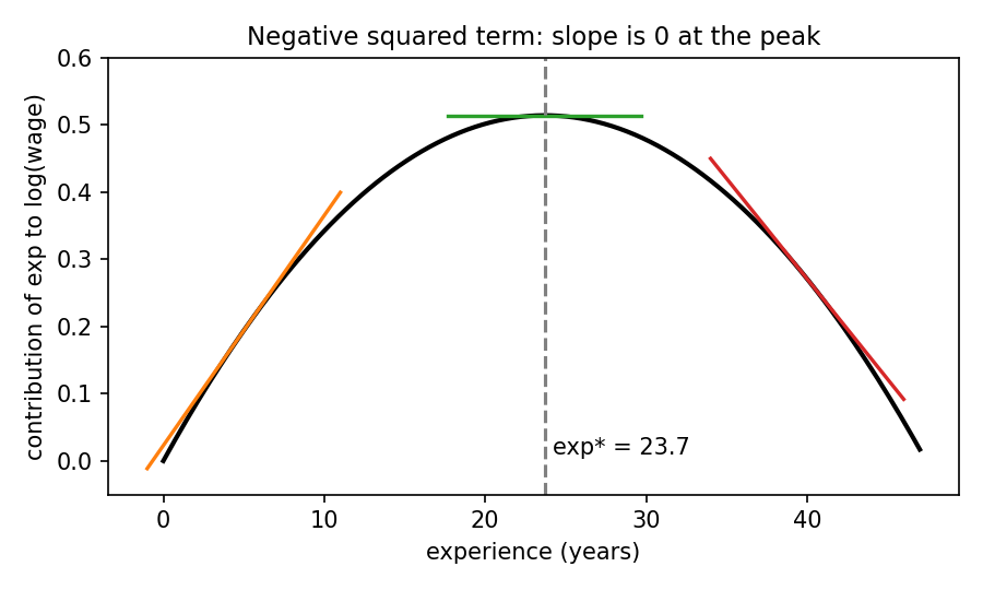
Reconstructed from the slidesThe figure is redrawn from the wage coefficients (slope lines at 5, 23.7 and 40 years). The lecture's own sketch labels the peak "23.68" while its algebra gives 23.698; I use 23.70.
Common mistakes
- Interpreting alone as "the effect of experience". With a square, the effect is and depends on the level of .
- Testing only or only to say "experience matters". Both belong to the same effect.
- Forgetting that a turning point may lie outside the observed range of the data (see the smoking example below).
Summary ruleA negative squared coefficient: the effect of goes up then down. A positive one: down then up.
3. Including an irrelevant variable
Suppose the true model has no ():
but we estimate .
- Unbiasedness is preserved: , , . The sample value will almost never be exactly 0 (that is just sampling noise), but its expectation is.
- Variance rises. Adding regressors does not bias estimates but inflates their variances, so coefficients can become insignificant.
Why variance rises (Activity 9 part 2)
Use .
| Case | What happens | Variance of the estimator |
|---|---|---|
| (a) correlated with | rises, so falls, the denominator shrinks | increases |
| (b) uncorrelated with | , so | equals , no loss |
Reconstructed from the slidesThe slide gives only the blanks and the formula; the filled-in answers above are the standard reading of that formula.
Diagnose and fix
- Easy to spot: the variance is high, so we cannot reject .
- Easy to fix: drop the variable and re-estimate.
- Example (slide 24),
price = b0 + b1 bdrms + b2 sqrft + uon HPRICE1:
| Term | Estimate | Std. error | t | p |
|---|---|---|---|---|
| (Intercept) | -19315.00 | 31046.62 | -0.622 | 0.536 |
| bdrms | 15198.19 | 9483.52 | 1.603 | 0.113 |
| sqrft | 128.44 | 13.82 | 9.291 | 1.39e-14 |
We cannot reject that or that the intercept is 0.
Check multicollinearity before dropping a variableHigh collinearity also gives small t-statistics, so a variable that looks irrelevant may be relevant but collinear with another. Look at the correlation matrix of the regressors first (slide 25).
4. Omitting a relevant variable
Why it is a big problem
- If the missing variable was never measured, it is hard to fix.
- The estimators are biased.
Setup. True model (1), satisfying Gauss-Markov A1 to A4 (see Gauss-Markov Theorem):
We wrongly estimate model (2), which omits :
The effect of is absorbed into . If and are correlated, then is correlated with , which violates A2, and is biased.
Derivation of the bias
Step 1. Substitute the true into the OLS formula for :
Since , the term vanishes, and the term simplifies to . So:
Step 2. Take expectations. The error term in model (1) satisfies A2, so the last fraction has expectation zero:
where is the sample covariance of and , and is the sample variance of . Hence:
Even a low correlation between and biases the estimate if is omitted.
Direction of the bias
| Bias in | ||
|---|---|---|
| upward | ||
| downward | ||
| downward | ||
| upward |
- ( uncorrelated): no bias.
- : the omitted variable was irrelevant after all.
- With several omitted variables the estimates are biased but the net direction is hard to know.
Variance when a variable is omitted
The earlier variance formula assumed unbiasedness, so it must be recalculated. The variance can be larger or smaller, and it is not informative when the estimator is biased. Recall that an efficient estimator has minimum variance among unbiased estimators.
Example: wage, education and IQ (slide 34)
| Model | Coefficient on educ | Std. error |
|---|---|---|
Omitted: lwage ~ educ |
0.059588 | 0.006809 |
Correct: lwage ~ educ + IQ |
0.040341 | 0.007996 |
Correlation of educ and IQ is 0.5429, and IQ has a positive effect on wage. Both signs are positive, so omitting IQ biases the education estimate upward, from about 4% to about 6%. Note the standard error was also smaller in the omitted model, yet that model is the wrong one.
Example: education and cigarettes (slides 36 to 43)
Regressing cigs ~ educ gives (se 0.1580, t = -1.38, p = 0.167): not significant. That estimate is unbiased only if educ is uncorrelated with other determinants of smoking sitting in the error.
| Pair | Correlation |
|---|---|
| educ, age | -0.181 |
| educ, lincome | 0.314 |
Both variables correlate with education. Adding age, agesq and lincome:
| Term | Estimate | Std. error | t | p |
|---|---|---|---|---|
| (Intercept) | -6.052 | 6.663 | -0.91 | 0.364 |
| educ | -0.515 | 0.167 | -3.08 | 0.002 |
| age | 0.780 | 0.161 | 4.86 | 0.000 |
| agesq | -0.009 | 0.002 | -5.21 | 0.000 |
| lincome | 0.734 | 0.727 | 1.01 | 0.313 |
residual df, . The education effect becomes significant: each extra year of education is associated with about half a cigarette fewer per day, so the earlier estimate was biased toward zero.
Quadratic in agePredictions at zero income and education (intercept plus age terms, as on the slide): age 30 gives 9.25, age 40 gives 10.75, age 60 gives 8.35 cigarettes per day. Peak smoking age: .
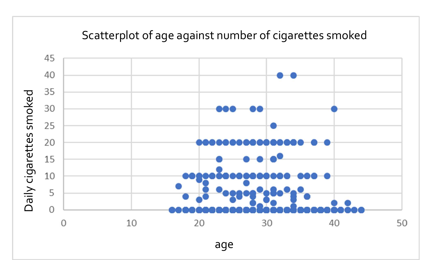
The scatterplot (slide 42) is how one might suspect a curve, but the picture is noisy: the data run only to about age 44, so the peak at 42.86 sits right at the edge of the sample.
Predictions at "no income, no education"The slide's predictions set education and income to zero and use
lincome=0(income of 1). That is an extrapolation, so treat the levels loosely; the shape in age is the point.
What if we omit age-squared? cigs ~ educ + age + lincome gives educ -0.390 (p = 0.021), age -0.043 (p = 0.134, not significant), lincome 1.753 (p = 0.014). Without the square we draw very different conclusions about age, and the educ estimate shifts again.
Included vs omitted: bias against variance
| Include irrelevant variable | Omit relevant variable | |
|---|---|---|
| Bias | none | yes: |
| Variance | higher | can be higher or lower; unreliable |
| Easy to detect? | yes (high se, insignificant) | no |
| Easy to fix? | yes (drop it) | only if the data exist |
Rule of thumb (slide 44)To decide whether to add a variable, weigh bias against variance. We always prefer unbiasedness over minimal variance, so we add any relevant explanatory variable.
5. Regression through the origin
Omitting the intercept biases the estimate unless the true intercept is zero. See Regression Through the Origin.
- The two slope estimates are equal only if .
- No-intercept OLS is unbiased only if the true .
- Allowing an intercept when is a small mistake: will be near zero and under A1 to A4 everything stays unbiased.
- Dropping the intercept when biases .
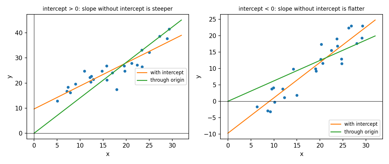
Reconstructed from the slidesThe lecture shows two schematic sketches (: ; : ). This figure re-simulates the idea with made-up points (true slope 1), so it shows direction only, not data.
From HW 4: consumption on GDP (slide 50)
Model Intercept Slope With intercept -2.189e+04 0.8155 (se 0.0191) Through origin none 0.51524 (se 0.00928) Negative , so . Note the no-intercept is not comparable to 0.9827.
Related work: Assign_04-Omitted Variables, F-tests & Multicollinearity (Birthweight & Soda Prices), Assign_05-Quadratics, Dummy Variables, Interactions & the Chow Test, Assign_03-Change of Variables, Regression Through the Origin & the Housing Model.
6. Practice exam questions (slides 51 to 71)
Activity 9 part 3: income and consumption (2018 Moed A, Question III)
Model: (model 3).
| Term | Estimate | Std. error | t | p |
|---|---|---|---|---|
| (Intercept) | -5.899e+04 | 7.170e+03 | -8.227 | 2.71e-09 |
| INCOME | 1.869 | 0.2020 | 9.251 | 1.99e-10 |
| INCOME2 | -7.272e-06 | 1.391e-06 | -5.227 | 1.12e-05 |
, 31 residual df. .
Q6: test a non-linear effect of income at 99%The slides leave this for the class; the working below is mine.
- a) against (two-sided).
- b) .
- c) Critical value: .
- d) : reject at 1%. Income has a non-linear effect on consumption.
High correlation of andThe correlation of 0.9975 is built in (a variable and its square rise together) and is not a problem for the squared term here; the coefficients are still highly significant.
Activity 9 part 4: housing prices
. Output: intercept 5.61070 (0.65128); lsqrft 0.70023 (0.09287, t = 7.540); llotsize 0.16797 (0.03828, t = 4.388); bdrms 0.03696 (0.02753, t = 1.342, p = 0.183). , adjusted 0.6302, residual se 0.1846 on 84 df, SSR = 2.862557.
Q1: is the price elasticity with respect to area one?
- , (in a log-log model is an Elasticity).
- .
- Critical value about 2 (5%, 84 df).
- : reject at 5%.
Q3: "the 85% confidence interval for bdrms will not include 0": correct?No. The p-value is 0.183, so we fail to reject at any . The interval contains 0 for all such , and for 85% . So 0 is inside the 85% interval and the researcher is wrong.
The link between CI and test (slides 61 to 62): the interval is with . We fail to reject at level iff lies in the interval. See Confidence Interval.
Q4: a linear restrictionClaim: adding to changes by four times as much as adding to .
Adding to changes by ; adding to changes it by . So .
- a) (equivalently ).
- b) Unrestricted: the full model above.
- c) Restricted: substitute : .
- In R: dependent variable
lprice; regressorsbdrmsand a new variable .Test with the F-test comparing restricted and unrestricted SSR.
Q5: , other assumptions hold
- Estimators unbiased.
- Variance minimal and estimators efficient: high (not perfect) correlation inflates the variance relative to uncorrelated regressors, yet the Gauss-Markov theorem still holds, so OLS has minimum variance among unbiased linear estimators. This is the slide's answer; the reason is my wording.
Q6: omit because of the high correlation (model 2)Model (2): . Output: intercept 6.28435 (0.69758); lsqrft estimate and se hidden on the slide, t = 8.190; bdrms 0.03811 (0.03034, t = 1.256, p = 0.213).
- a) Biased: is relevant (, highly significant) and correlated with , so omitting it gives omitted variable bias.
- b) Variance not necessarily minimal.
- c) Not efficient.
- d) "The elasticity with respect to area in (2) is greater than 0.7": the slide shows no marked answer. Since and the correlation is positive, the bias is upward, so the estimate in (2) should exceed 0.70023, but the actual estimate is hidden. Reconstructed, unsure: I would answer "we cannot say" about the true elasticity (a biased estimate does not tell us the truth); an examiner might accept TRUE if asked about the estimate itself.
Past-paper practice for the same ideas: Lec_13-Exam Review.
Summary
- Misspecification has two forms: adding an irrelevant variable or omitting a relevant one.
- A squared term gives a parabola; the marginal effect is and the peak or trough is at .
- Irrelevant variable: unbiased but higher variance; easy to spot and fix, but check multicollinearity first.
- Omitted variable: biased by ; sign from the signs of and ; variance no longer reliable; hard to detect and fix. Prefer unbiasedness over small variance, so include relevant variables.
- No intercept biases the slope unless or ; including an unneeded intercept is harmless.
- A CI and a two-sided test are the same thing: reject at iff is outside the interval.
Related notes
- Hub: Intro Econometrics
- Previous: Lec_08-Goodness of Fit & Multicollinearity — goodness of fit and multicollinearity
- Next: Lec_10-Dummy Variables — dummy variables, then Lec_11-Interaction Terms and Lec_12-Heteroskedasticity
- Course review: Lec_13-Exam Review
- Concepts: Model Misspecification, Omitted Variable Bias, Quadratic Model, Marginal Effect, Regression Through the Origin, Multicollinearity, Variance of the OLS Estimator, Gauss-Markov Theorem, F-test, Confidence Interval, Elasticity
- Assignments: Assign_03-Change of Variables, Regression Through the Origin & the Housing Model, Assign_04-Omitted Variables, F-tests & Multicollinearity (Birthweight & Soda Prices), Assign_05-Quadratics, Dummy Variables, Interactions & the Chow Test