
Heterogeneity, Inequality & Polarization
- #macroeconomics
- #inequality
- #polarization
- #heterogeneity
- #skill-biased-technological-change
- #routine-biased-technological-change
- #automation
- #task-based-model
- #labor-share
Heterogeneity, Inequality & Polarization
Part of: Macro-Economics Lecture 09 — Macro-Economics, "Heterogeneity, Inequality, and Polarization in the Labor Market" Key concepts: Heterogeneity, Inequality Measures, Skill-Biased Technological Change, Polarization, Routine-Biased Technological Change, Task-Based Model, Automation, Labor Share
Where This Fits
The models so far (Lec_07-Labor Market, Lec_08-Labor Market Data, Participation & Unemployment) assumed homogeneous workers and firms — one representative worker, one wage. That is fine for aggregate responses but says nothing about distribution: who wins, who loses, and why inequality has changed.
This lecture introduces heterogeneity and asks what simple, tractable modifications of the standard labor model can explain the major empirical trends in inequality. The story moves in three stages:
- Skill-biased technological change (SBTC) — split workers into skilled/unskilled.
- Polarization — the middle hollows out; shift the lens from skill to tasks/occupations.
- Task-based models of automation — the modern framework, with displacement, productivity, and reinstatement effects.
An explicit caveat from the slidesSBTC and routinization are not the only explanations for inequality — they get attention because they are empirically important and require only simple extensions of the model we already have. This is a "scratch the tip of the iceberg" tour, focused on income (not wealth) inequality.
Why We Care About Heterogeneity
A representative-agent model cannot address:
- Distributional consequences of policy — the heart of Lec_10-Fiscal Policy analysis (and increasingly monetary policy too).
- Differences in behavior across households — e.g. heterogeneity in the marginal propensity to consume (MPC), which determines how much a stimulus or recession is amplified (the "matching multiplier").
- Sectoral trends — shifts across industries, education groups, and occupations that aggregates hide.
Measuring Inequality
Main data sources: the World Inequality Database (WID) and the Global Repository of Income Dynamics (GRID).
| Measure | Definition | Note |
|---|---|---|
| ==Gini coefficient== | Area between Lorenz curve and 45° line; = perfect equality, = perfect inequality | Most common single-number summary |
| Variance of log income | Decomposable into components | |
| Coefficient of variation | Rarely used | |
| Percentile ratios | 90/10, 90/50, 50/10 | Locate where in the distribution inequality lives |
Why the 90/50 and 50/10 split matters so muchBreaking the 90/10 ratio into an upper half (90/50) and a lower half (50/10) is the single most important diagnostic in this lecture. The two halves moved together in the 1980s but diverged afterward — and that divergence is exactly what motivates the shift from "skill" to "polarization."
The Lorenz curve underlying the Gini:
graph LR
    A["Cumulative % of population (x-axis)"] -->|"vs"| B["Cumulative % of income (y-axis)"]
    B --> C["45° line = perfect equality"]
    B --> D["Bowed curve = actual distribution"]
    D --> E["Gini = (area between line & curve)<br/>÷ (area under 45° line)"]
Stage 1 — Skill-Biased Technological Change (SBTC)
The Idea
Technology raises the productivity of skilled workers relative to unskilled workers, widening the wage gap. Empirically the college wage premium rose sharply: a coefficient of in a Mincer regression means — a college graduate earns ~97% more.
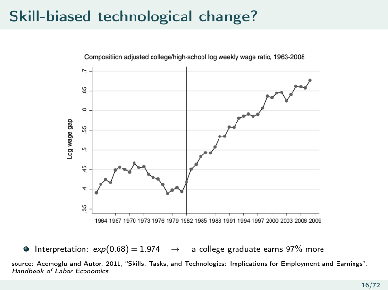 The college/high-school wage premium over time (Acemoglu & Autor 2011). The rising gap is the classic SBTC fact.
A Simple Model
Take two types of labor — skilled and unskilled — that are substitutes in production. Modify the production function to a nested CES form:
Under the parameter restriction :
- and are substitutes.
- A rise in skilled productivity increases but decreases .
Two Segmented Markets
Treat skilled and unskilled labor as two separate markets (extreme assumption: each worker participates in only one). A positive shock shifts only the skilled labor-demand curve:
graph TD
    subgraph "Skilled market"
    S1["A_s ↑ → MPN_s ↑"] --> S2["N^D_s shifts RIGHT"]
    S2 --> S3["w_s ↑ and N_s ↑"]
    end
    subgraph "Unskilled market"
    U1["A_s ↑ → MPN_u ↓"] --> U2["N^D_u shifts LEFT"]
    U2 --> U3["w_u ↓ and N_u ↓"]
    end
Result of the SBTC modelA positive skill-biased shock raises both employment and wages of skilled workers and lowers both for unskilled workers — generating wage inequality and differential employment from one simple parameter change. Consistent with the 1980s data.
But is it really only about skill?Did the effect of skill change over time? The next section says yes — after ~1990 the simple skill story breaks down, which forces a richer framework.
Stage 2 — Polarization
The Empirical Turn
From the 1990s, the simple SBTC story fits less well:
- Inequality kept widening in the upper half (90/50 keeps rising)…
- …but stopped widening in the lower half (50/10 flat or shrinking).
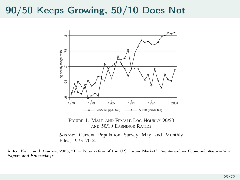 90/50 and 50/10 log earnings ratios (Autor, Katz & Kearney 2006). The two halves track together through the 1980s, then diverge — the upper half keeps climbing while the lower half stalls.
Simultaneously, employment grew at the top and bottom of the skill distribution but shrank in the middle — the hollowing-out called ==polarization==.
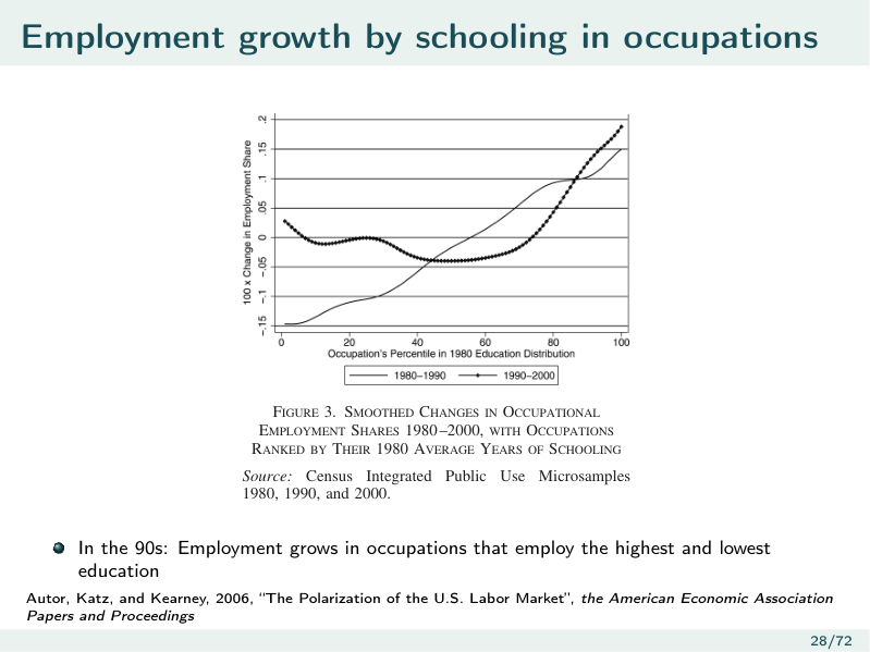 Smoothed employment-share growth by occupational skill percentile (Autor, Katz & Kearney 2006). The 1980s line is roughly monotonic in skill; the 1990s line is U-shaped — the signature "polarization curve."
What polarization forces us to doA monotonic "more skill = better" story (SBTC) cannot produce a U-shape. Polarization shifts the discussion from education/skill to occupation/task, and ties directly to automation, robots, and AI.
The Occupational Bar Chart
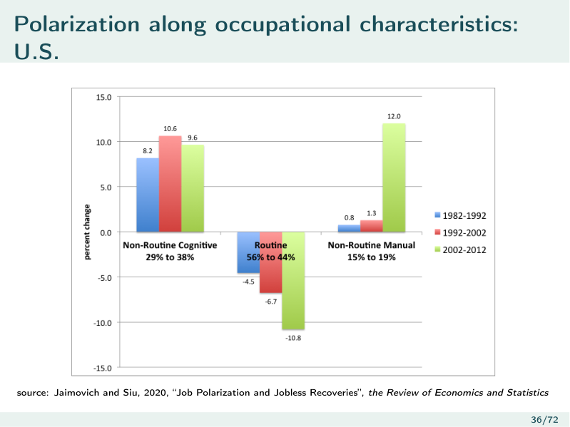 Percent change in employment shares by occupation group (Jaimovich & Siu). Middle-skill routine occupations shrink; non-routine cognitive (top) and non-routine manual (bottom) grow.
Stage 3 — Routinization & the Task Framework
Classifying Occupations
Occupations are split along two dimensions (Autor, Levy & Murnane 2003; Acemoglu & Autor 2011):
| Routine (follows explicit rules) | Non-routine (needs flexibility, creativity, interaction) | |
|---|---|---|
| Cognitive | Routine Cognitive (RC): bookkeepers, bank tellers, clerks, data entry | Non-routine Cognitive (NRC): managers, analysts, programmers, economists |
| Manual | Routine Manual (RM): machine operators, assemblers, fabricators | Non-routine Manual (NRM): janitors, home-care aides, bartenders, hairstylists |
The central hypothesis — "routinization"Computers (and capital generally) are close substitutes for routine tasks (which can be codified into rules) and complements to non-routine tasks. So technological progress displaces the routine middle (RC + RM) while raising demand at both ends (NRC at the top, NRM at the bottom) — producing polarization. Offshoring of routine work reinforces this.
The BLS Occupational Outlook data make it concrete: routine middle jobs (metal/plastic machine workers, office clerks, travel agents) are projected to decline ~6%, while non-routine jobs at both ends (home-health aides +21%, software developers +17%, economists higher pay) grow.
A Simple Automation Model
Let routine hours and non-routine hours enter production, with computer capital a substitute for routine labor:
Labor demand = marginal products:
The differential effect of more computer capital is the whole point:
Falling computer prices, step by step
- The price of computer capital falls → firms buy more .
- More lowers → routine labor demand falls → down.
- More raises → non-routine labor demand rises → up. Result: wages diverge between routine and non-routine work — polarization. (Supply also responds, so this is suggestive, not a full equilibrium solution.) Empirically, the prices of robots and ICT capital have fallen dramatically, matching the model's trigger.
The Task-Based Model of Production
A more flexible alternative: total output is a sum (or aggregate) of tasks, and each task can be produced by either capital or labor.
For task :
where , are labor and capital productivity in task . With wage and capital rent , the unit cost of task is with labor and with capital. The firm picks the cheaper:
graph LR
    T["Tasks ranked by comparative advantage"] --> C["Low-j tasks: capital cheaper → automated"]
    T --> L["High-j tasks: labor cheaper → done by workers"]
    C --> TH["Threshold task ĵ where w/ψ_N = r/ψ_K"]
    L --> TH
Three Effects of Better Capital
| Effect | What happens | Wage impact |
|---|---|---|
| Productivity effect | Capital gets cheaper/better at a task → cost of output falls; if the task allocation doesn't change, workers are better off (same wage, lower prices) | Wage ↑ (real) |
| Displacement effect | A task crosses the threshold and is reallocated from labor to capital | Wage ↓ |
| Reinstatement effect | New tasks are created, a subset performed by labor (occupations that didn't exist before) | Wage ↑ |
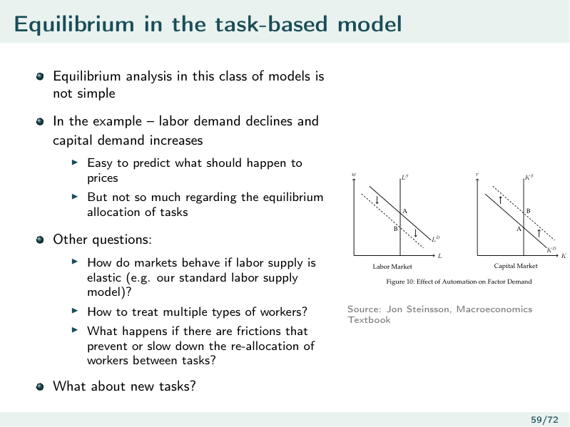 Effect of automation on factor demand (Steinsson textbook). Automation of a labor task shifts labor demand left (↓) and capital demand right (↑); displaced workers compete for remaining jobs, pushing wages down further before adjustment.
The pie can grow while labor's slice shrinksAutomation can raise total output (productivity effect) yet leave labor worse off if displacement outweighs productivity and reinstatement. Whether a given innovation helps or hurts workers depends on the balance of the three effects — the task model captures this richness that Cobb-Douglas/CES cannot.
New Tasks & Long-Run Growth
Long-run growth involves continual destruction and creation of tasks — old tasks automated away, new tasks (reinstatement) created for labor. The historical shift of workers across agriculture → manufacturing → services is the macro footprint of this churn.
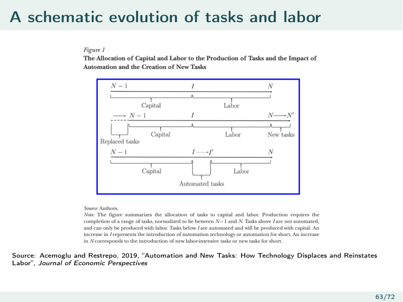 Schematic evolution of tasks and labor (Acemoglu & Restrepo 2019): automation displaces labor from old tasks while new tasks reinstate it.
Connection to the Declining Labor Share
The ==labor share== is the fraction of total income paid as wages. It has declined in recent decades (Israel, OECD). Acemoglu & Restrepo (2019) decompose the effect of automation on labor demand into:
Plus an aggregate composition effect — economic activity shifting across industries. The empirical decompositions (US 1947–1987 vs. 1987–2017) show reinstatement weakening and displacement strengthening in the later period — a plausible driver of the falling labor share.
Polarization & Policy
The trends are politically charged, so economists use models to weigh policy costs and benefits. To evaluate policy we need to know what happens to displaced routine (R) workers — do they end up working, in R again, in low-skill service (NRM), in high-skill (NRC), or out of the labor force (NLF)?
The data (Jaimovich, Saporta-Eksten, Siu & Yedid-Levi 2021) show, for low-skilled US workers: a ~16 percentage-point drop in routine employment, split roughly 2/3 into Not-in-Labor-Force and 1/3 into non-routine manual service jobs. Same pattern for men, women, and low-cognitive-ability groups.
Two policy families:
- Retraining — move displaced workers into growing occupations.
- Redistribution — transfer to the losers.
Policy findingsA few policies are aggregate welfare-improving, but none is Pareto-improving — there are always losers. Details matter enormously: who gets treated and how programs are financed change the verdict. Models are essential precisely because the trade-offs are not obvious.
Summary
- Representative-agent models can't address distribution; we add heterogeneity to study inequality and the differential effects of policy (including MPC heterogeneity).
- Inequality measures: Gini, variance of log, percentile ratios. The 90/50 vs. 50/10 split is the key diagnostic.
- SBTC: skilled and unskilled are substitutes; rising raises / and lowers /. Fits the 1980s and the rising college premium.
- After ~1990, polarization: upper-half inequality keeps rising while the lower half stalls; employment grows at top and bottom, shrinks in the routine middle — a U-shape SBTC can't explain.
- Routinization: computers substitute for routine tasks and complement non-routine ones, displacing the middle. Shifts the lens from skill to tasks/occupations.
- Simple automation model: more computer capital lowers and raises → wage divergence.
- Task-based model: each task done by cheaper of capital/labor; automation has productivity (+), displacement (−), and reinstatement (+) effects — output can grow while labor's share falls.
- Explains the declining labor share; policy can raise aggregate welfare but never Pareto-improves — there are always losers, and design details matter.
Related Notes
- Built on: Lec_07-Labor Market — the homogeneous labor model being relaxed;
- Built on: Lec_08-Labor Market Data, Participation & Unemployment — measurement, NLF margin (where displaced workers go)
- Built on: Lec_04-Production — production function, CES, Cobb-Douglas; the basis for SBTC and task models
- Companion: Lec_10-Fiscal Policy — distributional analysis where heterogeneity is essential
- Concept: Skill-Biased Technological Change, Routine-Biased Technological Change, Task-Based Model, Labor Share, Automation