Week 5

Investment

Part of: Macro-Economics Lecture 05 — Macro-Economics Key concepts: Capital Accumulation Equation, User Cost of Capital, Marginal Product of Capital, Depreciation, Two-Period Firm Problem

Where This Fits

We now have supply ( $Y$ from the production model) and consumption ( $C$ from Lec 02). The next component of demand is:

Y = C + \underbrace{I}_{\text{this lecture}} + G

Investment is how firms decide to accumulate capital — the same capital $K$ that drives output in the production function.

Why Investment Matters — The Data

Investment is 15–25% of GDP for most developed economies. But its importance goes beyond its size:

Feature	Detail
Links spending to growth	Investment today = capital tomorrow → drives future output
Highly volatile	≈ 4× as volatile as GDP — swings far more in recessions/booms
Leads the cycle	Investment often peaks or troughs slightly before GDP — a forecasting signal

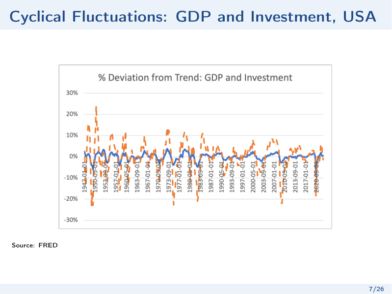l5_investment_cyclical Cyclical components of GDP and investment, USA. Investment swings far more violently than GDP (~4×) and often turns slightly ahead of it — hence its outsized role in the business cycle.

Why is investment so volatile?

Consumption is smoothed (see Lec 02 — the PIH/LCH). Investment has no such smoothing mechanism: firms can freely choose to invest a lot or very little depending on their expectations of future productivity and the real interest rate. This is why investment drives most of the cycle.

What counts as investment?

Category	Examples
Business fixed investment	New equipment, software, factories, office buildings
Residential investment	New homes and apartments
Change in inventories	Finished goods not yet sold (usually small)

Investment and Capital: The Accumulation Equation

==Capital accumulation equation== (the most important equation in this lecture):

\boxed{K_{t+1} = (1 - \delta)K_t + I_t}

$K_t$ = capital stock at the start of period $t$
$\delta$ = ==depreciation rate== — the fraction of capital that wears out each period (e.g. $\delta = 0.05$ means 5% of machines break down or become obsolete each year)
$I_t$ = new investment during period $t$
$K_{t+1}$ = capital available next period

Interpretation: next period's capital = surviving old capital + new investment.

To keep capital constant (no growth), invest just enough to replace what depreciates:

\bar{I} = \delta \bar{K}

Investment vs. capital — don't confuse them

Capital ( $K$ ) is a stock: how much machinery exists right now. Investment ( $I$ ) is a flow: how much new machinery is purchased this period. Investment adds to the capital stock; depreciation subtracts from it. The analogy: water in a bath (capital), the tap (investment), and the drain (depreciation).

This creates an intertemporal dimension: investing today pays off in the future, not immediately. So firms must solve a multi-period optimisation problem.

The Firm's Optimisation Problem

Setup

Firms own capital (they don't rent it). Their profits in any period are:

\Pi_t = \underbrace{Y_t}_{\text{revenue}} - \underbrace{w_t N_t}_{\text{labour cost}} - \underbrace{p_{k,t} I_t}_{\text{investment cost}}

where $p_{k,t}$ is the price of capital goods relative to consumption goods.

Using the accumulation equation, we can rewrite investment in terms of capital:

I_t = K_{t+1} - (1-\delta)K_t

So the firm is really choosing how much capital to have next period ( $K_{t+1}$ ).

We also allow for a corporate tax rate $\tau_k$ on profits:

\Pi_t = (1-\tau_k)(Y_t - w_t N_t) - p_{k,t}(K_{t+1} - (1-\delta)K_t)

Note: the tax only applies to operating profits, not the capital expenditure itself.

Two-Period Problem

Consider a firm that lives for two periods (current = 0, future = 1). Firms discount future profits by $\frac{1}{1+r}$ (the same real interest rate that consumers face). The firm's problem is:

\max_{N_0, N_1, K_1, K_2} \left\{ (1-\tau_k)(A_0 F(K_0,N_0) - w_0 N_0) - p_{k,0}(K_1-(1-\delta)K_0) \right.

\left. + \frac{1}{1+r}\left[(1-\tau_k)(A_1 F(K_1,N_1) - w_1 N_1) - p_{k,1}(K_2-(1-\delta)K_1)\right] \right\}

Boundary condition: $K_2 = 0$ (finite horizon — the firm doesn't need capital beyond the last period).

First-Order Conditions

For labor (same in both periods): factors paid their marginal products:

\text{MPN}_0 = w_0, \qquad \text{MPN}_1 = w_1

For capital ( $K_1$ ): equate the cost of investing today to the discounted benefit of having more capital tomorrow:

p_{k,0} = \frac{1}{1+r}\left[(1-\tau_k)\cdot\text{MPK}^f + p^f_k(1-\delta)\right]

Using superscript $f$ for future-period variables:

\boxed{p_k = \frac{1}{1+r}\left[(1-\tau_k)\,\text{MPK}^f + p^f_k(1-\delta)\right]}

The User Cost of Capital

Rearranging the FOC to isolate $\text{MPK}^f$ :

\boxed{\text{MPK}^f = \underbrace{\frac{(1+r)\,p_k - (1-\delta)\,p^f_k}{1-\tau_k}}_{\text{user cost of capital}}}

The ==user cost of capital== is the effective cost of using one unit of capital for one period. It has three components:

Component	Formula	Intuition
Financing cost	$r \cdot p_k$	You either borrow to buy capital (pay interest) or forego the return on savings
Depreciation	$\delta \cdot p^f_k$	Capital wears out; you lose a fraction each period
Capital gain/loss	$p_k - p^f_k$	If capital prices fall, owning capital is more expensive in real terms
Tax wedge	$\div (1-\tau_k)$	Corporate taxes reduce the net return, so you need a higher gross MPK to break even

The machine analogy

Imagine you own a machine. You could instead:

Use it → generates MPK $^f$ extra output

Sell it, put the money in the bank → earn $r \cdot p_k$ in interest, then (try to) buy it back next year

The user cost captures option 2. Firms invest until the return on capital equals the cost of using it.

The Investment Decision — Graphically

The optimal level of future capital $K^f$ is where:

\text{MPK}^f = \text{user cost}

Since $\text{MPK}^f$ is decreasing in $K^f$ (diminishing marginal product), but the user cost is flat (it doesn't depend on $K^f$ — all components are exogenous to the firm), there is a unique crossing point.

type: production-capital
figure: user-cost

The optimal capital stock sits where the downward-sloping $MPK^f$ curve crosses the flat user-cost line. A higher $r$ , $p_k$ , or $\delta$ raises the user cost (line up → less capital); a higher $A^f$ or $N^f$ raises $MPK^f$ (curve out → more capital).

Investment follows from the optimal $K^f$ :

I = K^f - (1-\delta)K

If desired $K^f >$ current $K$ (adjusted for depreciation), invest. Otherwise, disinvest (let capital depreciate).

Comparative Statics

What happens to optimal $K^f$ and investment $I$ when each variable changes?

Variable changes	Effect on user cost	Effect on MPK $^f$	Effect on $K^f$	Effect on $I$	Intuition
$r$ ↑	↑	—	↓	↓	Funding capital is more expensive; discount future returns more heavily
$A^f$ ↑	—	↑	↑	↑	Capital is more productive in the future
$p_k$ ↑	↑	—	↓	↓	Capital goods are more expensive to buy
$p^f_k$ ↑	↓	—	↑	↑	Future capital is more valuable; buying now is relatively cheaper
$\delta$ ↑	↑	—	↓	↓	Faster depreciation — less capital survives, so you effectively pay more to maintain a given stock
$N^f$ ↑	—	↑	↑	↑	Complementarity: more future labour → higher MPK $^f$
$A$ ↑ (current)	—	—	—	—	Only current output changes, not future MPK — no effect on investment

Current vs. future TFP

A rise in current $A$ does not shift the investment curve — investment depends on the future marginal product of capital. Only a rise in future $A^f$ stimulates investment. This distinction is critical for the goods market analysis in Lec 06.

Numerical Example

Given:

$Y = A \cdot K^{0.5} N^{0.5}$ , so $\text{MPK}^f = 0.5 \cdot A^f (K^f)^{-0.5} (N^f)^{0.5}$
$A^f = 200$ , $N^f = 100$ , $K = 300$
$p_k = p^f_k = 500$ , $r = 0.05$ , $\delta = 0.05$ , $\tau_k = 0$

Step 1 — User cost:

\frac{(1+0.05)\times 500 - (1-0.05)\times 500}{1} = \frac{525 - 475}{1} = 50

Step 2 — MPK $^f$ :

\text{MPK}^f = 0.5 \times 200 \times (K^f)^{-0.5} \times 100^{0.5} = \frac{1000}{\sqrt{K^f}}

Step 3 — Set MPK $^f$ = user cost:

\frac{1000}{\sqrt{K^f}} = 50 \implies \sqrt{K^f} = 20 \implies K^f = 400

Step 4 — Find I:

I = K^f - (1-\delta)K = 400 - (0.95)(300) = 400 - 285 = 115

Check the intuition

Current capital is 300. After depreciation: $0.95 \times 300 = 285$ . The firm wants 400, so it needs to invest 115 to make up the difference.

Summary

Capital accumulation: $K_{t+1} = (1-\delta)K_t + I_t$ . Investment adds to the capital stock; depreciation subtracts.
Firm's problem: maximise multi-period profits by choosing how much capital to hold each period.
Optimality condition: MPK $^f$ = user cost of capital. Invest until the marginal return on capital equals the effective cost of using it.
User cost = interest cost + depreciation + price changes, scaled by the tax wedge.
Key comparative statics: higher $r$ or $p_k$ → less investment; higher $A^f$ , $N^f$ , or $p^f_k$ → more investment. Current TFP has no effect.

Built on: Lec_04-Production — production function, MPK, complementarity
Companion: Lec_02-Consumption and Saving — the household side of the same intertemporal problem
Next: Lec_06-Equilibrium in the Goods Market — combines S and I to determine equilibrium r
Future: Lec_07-Labor Market — uses MPN = w condition from the same firm problem

Investment

Investment

Where This Fits

Why Investment Matters — The Data

What counts as investment?

Investment and Capital: The Accumulation Equation

The Firm's Optimisation Problem

Setup

Two-Period Problem

First-Order Conditions

The User Cost of Capital

The Investment Decision — Graphically

Comparative Statics

Numerical Example

Summary

Related Notes