
Macro Data Review
- #macroeconomics
- #gdp
- #gni
- #inflation
- #price-index
- #business-cycles
- #real-vs-nominal
- #exchange-rates
- #fisher-equation
Macro Data — A Review
Part of: Macro-Economics Key concepts: GDP, GNP, Real vs Nominal, GDP Deflator, CPI, Business Cycles, Fisher Equation, Purchasing Power Parity
Measurement of Economic Activity
Three equivalent approaches to measuring the size of an economy:
| Approach | What it counts |
|---|---|
| Product | Value added — output minus intermediate inputs |
| Income | Wages + capital income + firm profits |
| Expenditure | Total spending by final purchasers |
The core identityEvery unit of output produced is purchased by someone and generates income for someone. The three approaches are just different accounting views of the same circular flow.
graph LR
    F[Firms<br/>produce output] -->|goods & services| H[Households]
    H -->|spending = Expenditure| F
    F -->|wages, profits, rent = Income| H
    P([Product / Value Added]) -.equal.- I([Income])
    I -.equal.- E([Expenditure])
    class F,H internal-link;
The circular flow: the same money measured at three points — output sold, income paid, spending received.
Gross Domestic Product (GDP)
GDP is the single most-used measure of economic activity — correlated with standard of living, unemployment, fiscal deficits, and inflation.
The national accounts identity
Expenditure components
- — households buying new goods and services.
- — capital used for future production (including inventory changes).
- — government purchases of goods and services (excludes transfer payments).
- — exports minus imports.
Value added vs. final goods
Coffee chainFarmer sells beans for $1 → roaster sells for $2.20 → shop sells espresso for $3.
Stage Value added Farmer $1 Roaster $1.20 Coffee shop $0.80 Sum $3 The final good is the $3 espresso. GDP = $3 by both the value-added and expenditure approach. Don't double-count intermediates.
GDP vs. GDI — Do Approaches Align?
GDI (Gross Domestic Income) should equal GDP in theory. In practice (US, 1947–2025), discrepancies are not small and come from:
- Government transfers (e.g., COVID-era stimulus mismeasurement).
- Corporate earnings bursts.
- Individuals misreporting (e.g., booking capital gains as income).
Which to use?Customarily we use GDP, but an emerging suggestion is to average the two. Recent debate: GDI has run above trend while GDP has run below — the gap matters for policy.
What GDP is NOT
- Not easily comparable across countries — population size and purchasing-power differences distort raw comparisons.
- Not a measure of everything valuable — excludes:
- Home production, black-market activity
- Environmental quality, crime/safety
- Income (in)equality
- Not welfare — in theory we'd measure welfare with a utility function; GDP is just a (strongly correlated) proxy.
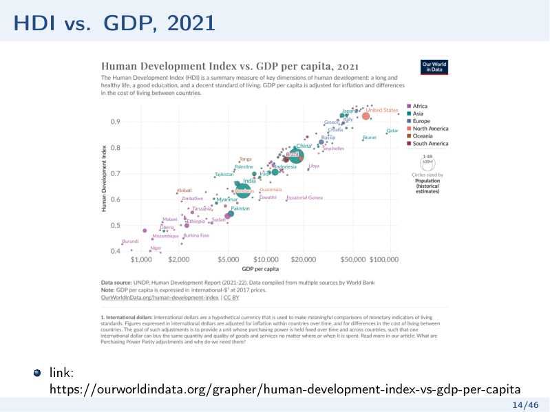 HDI vs. GDP per capita across countries (2021). Strongly correlated, but with wide dispersion — many countries sit well above or below the income-predicted line.
The Human Development Index (HDI)
Still criticised (why those three? why equal weights?) but a better proxy for living standards than GDP alone.
Jones & Klenow (2016)
Model-based welfare measure integrating consumption + leisure + life expectancy + inequality. Inequality matters "behind the veil of ignorance" — captures risk faced by a randomly-drawn citizen.
- Finding 1: welfare and income are highly correlated.
- Finding 2: but with huge dispersion around the 45° line — many countries are richer or poorer in welfare terms than their GDP suggests.
Nominal vs. Real GDP
Why the distinction matters
Nominal GDP for period :
If nominal GDP rises, we can't tell whether quantities grew, prices grew, or both. Real GDP strips out price changes to isolate quantity changes.
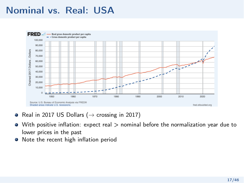 Nominal vs. real GDP, USA (real in 2017 dollars, so the lines cross in 2017). With positive inflation, nominal sits above real after the base year and below it before.
Fixed-weight real GDP
Pick a base year, fix prices at that year's level, let quantities vary.
Base year = 2010
Year Nominal GDP Real GDP (2010 $) 2010 $12,000 $12,000 2020 $22,500 $19,000 Growth 87.5% 58.3% Base year = 2020 instead gives real growth of 60.71% — different answers from the same data!
The base-year problemChoice of base year materially changes growth estimates, especially when relative prices shift quickly. A partial fix: chain-weighting.
Chain-weighted growth rate
Geometric average of growth rates computed with both years' prices:
In the example above: — smoothly between the two fixed-weight answers.
Building real GDP from chain-weighted growth rates:
Average Growth Rates
Geometric average over periods with constant growth :
Doubling in 40 years, : .
Catch-up / doubling questions
Given , how long to multiply output by factor ?
Used to answer "if two countries grow at different rates, will they ever converge?" — substitute in the ratio you want and solve for .
GDP vs. GNP
- GNP = income earned by the nation's factors of production, wherever located.
- GDP = income earned by factors located within the domestic economy, regardless of nationality.
where (Net Factor Payments) = payments from abroad to domestic citizens minus payments to foreigners residing domestically.
The Ireland case (2019)Ireland's GNP was 21% below its GDP because of foreign multinationals booking profits there. For small open economies with heavy foreign-owned capital, GDP overstates the income that actually flows to nationals.
Business Cycles — Trend vs. Cycle
Each observation decomposes into:
Extracting the trend — HP filter
Use the Hodrick–Prescott filter with smoothing parameter (quarterly data). Other methods (band-pass, one-sided filters) give similar pictures.
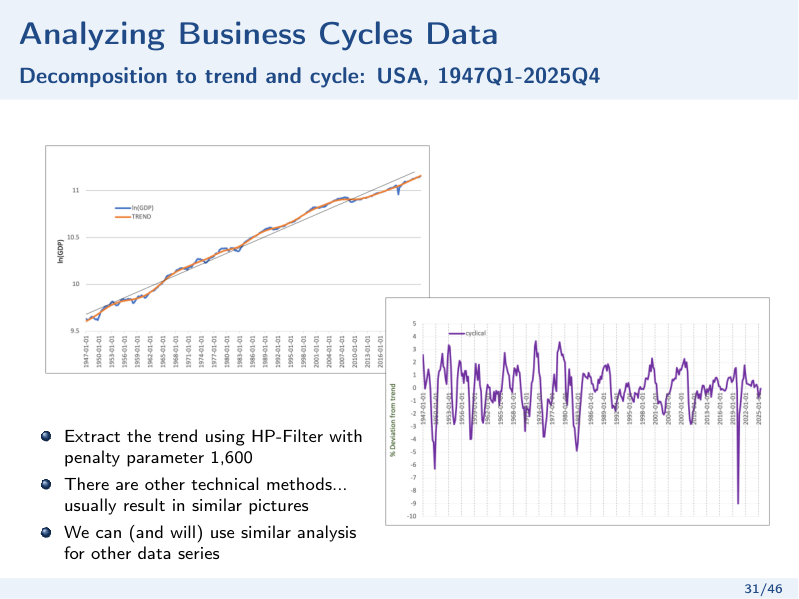 Trend/cycle decomposition of US log GDP (HP filter, λ=1,600). Top: log GDP vs. its smooth trend. Bottom: the cyclical component — deviations from trend that define booms and recessions.
Cyclical diagnostics
Once we have , compute its correlation with other series' cyclical components:
| Correlation sign | Label |
|---|---|
| Pro-cyclical (e.g., consumption, investment) | |
| Counter-cyclical (e.g., unemployment) | |
| Acyclical |
Also compare standard deviations: durables fluctuate more than non-durables; investment fluctuates much more than consumption.
Recurring toolkitThese cyclical statistics (correlation with GDP + relative volatility) are used throughout the course — see Lec_02-Consumption and Saving for the stylised facts on .
Price Indexes and Inflation
Definitions
A price index is the average price level of a basket relative to a base year. Inflation is the percentage change in the index:
The GDP deflator
Depends on the choice of base year and weighting rule (fixed vs. chain-weighted).
Consumer Price Index (CPI)
Current price of a fixed consumption basket relative to its base-year price. Three practical problems:
- Picking the representative basket — it evolves over time and across regions.
- Quality improvements — is last year's phone "the same good" as this year's?
- New products — how to introduce them into the basket.
Personal Consumption Expenditure (PCE) deflator
Like the GDP deflator for the consumption sub-aggregate, but with a changing basket (unlike fixed-basket CPI).
Which index covers what?
| Measure | Capital goods | Imports | Basket |
|---|---|---|---|
| GDP deflator | ✅ (if home-produced) | ❌ | Changes implicitly |
| CPI | ❌ | ✅ | Fixed |
| PCE deflator | ❌ | ✅ | Changes |
Exchange Rates and Purchasing Power
The problem
GDP is measured in local currency. To compare across countries we need a common unit — typically USD. But the nominal exchange rate (e.g., ~3.1 ILS per USD) does a poor job reflecting differences in what the money can buy.
Purchasing Power Parity (PPP)
Compare the cost of the same basket in local currency across countries:
Then convert to common units:
Data source: Penn World Tables.
The comparability problem never goes fully awayHow do we know the "representative basket" is really the same in two different countries? Different datasets can give quite different PPP numbers.
Nominal and Real Interest Rates
The Fisher equation
where = nominal rate, = inflation, = real rate. The approximation holds when are small.
Ex-post vs. ex-ante
Ex-post (realised): use actual inflation. Ex-ante (expected):
What households and firms actually care about when making decisions — the expected real return.
Interest rates are pricesAn interest rate is the price of moving consumption (or capital) across time. This frames the whole Lec_02-Consumption and Saving problem — the real interest rate is the price that appears in the Euler equation.
Summary — What This Lecture Teaches
- GDP = income = expenditure — three equivalent measurement approaches, with non-trivial discrepancies in practice (GDP vs. GDI).
- GDP is a proxy for welfare, not welfare itself — HDI and Jones–Klenow give richer pictures.
- Real vs. nominal matters: fixed-weight indexes are base-year sensitive; chain weighting is the standard fix.
- Average growth rates use geometric means; the formula answers catch-up and doubling questions.
- GNP vs. GDP can diverge sharply for small open economies (Ireland).
- Business cycles are deviations from an HP-filtered trend; cyclical correlation + relative volatility are the core diagnostics.
- GDP deflator, CPI, PCE deflator differ in basket coverage (capital goods, imports) and weighting rules.
- PPP exchange rates beat nominal rates for cross-country comparison, but aren't perfect.
- Fisher equation connects nominal and real rates — the real rate is the relevant price for intertemporal decisions.
Related Notes
- Companion: Lec_02-Consumption and Saving — uses the cyclical facts established here
- Foundational: National Accounts, HP Filter, Inflation, Exchange Rates
- Future applications: Fiscal Policy, Monetary Policy, Growth Models