
Labor Market Data, Participation & Unemployment
- #macroeconomics
- #labor-market
- #unemployment
- #participation
- #labor-force
- #search-frictions
- #stocks-and-flows
Labor Market Data, Participation & Unemployment
Part of: Macro-Economics Lecture 08 — Macro-Economics, "The Labor Market, Part II" Key concepts: Unemployment Rate, Labor Force Participation, EPOP, Sticky Wages, Frictional Unemployment, Stocks and Flows Model, Job Finding Rate, Separation Rate
Where This Fits
Lec_07-Labor Market built a frictionless labor market: every worker willing to work at the market wage finds a job, so there is no unemployment in equilibrium. That is useful for thinking about employment quantities over the cycle, but it cannot speak to the thing people actually care about — unemployment.
This lecture does two things:
- Measurement — the labor-market "aggregates" (, , participation) are subtler than GDP because they come from surveys and depend on definitions. We need to know what the numbers mean before we model them.
- A first model of unemployment — since the baseline model generates none, we bolt on a simple two-state stocks-and-flows description driven by a ==job-finding rate == and a ==separation rate ==. This is the gateway to modern search-and-matching theory.
Where the Data Comes From
Labor-market aggregates are survey-based, not administrative counts. In the US:
| Survey | Unit | Size | Measures |
|---|---|---|---|
| Current Population Survey (CPS) | Households | ~60,000 households | Unemployment rate, participation, flows |
| Current Employment Statistics (CES) | Businesses / establishments | ~121,000 firms & gov't agencies, ~631,000 worksites | Net job gain/loss, payroll employment |
Household vs. establishment surveys can disagreeBecause the two surveys sample different units (people vs. firms), they can paint different pictures of the same month — a recurring headache when reading "the jobs report."
The Three Labor-Market States
Every person aged 15+ is classified into exactly one of three groups:
graph LR
    POP[Working-age population<br/>15+] --> E[Employed E<br/>worked last week]
    POP --> U[Unemployed U<br/>no work, actively searched<br/>last 4 weeks, available]
    POP --> NLF[Not in Labor Force NLF<br/>students, retirees, etc.]
    E -.->|Labor Force = E + U| LF[Labor Force]
    U -.->|Labor Force = E + U| LF
    class E,U,NLF internal-link;
- ==Employed (E)== — worked full- or part-time during the past week (or was on sick leave, vacation, or strike).
- ==Unemployed (U)== — without work, actively sought work in the past four weeks, and available for work. This active-search requirement is exactly what the frictionless model is missing.
- ==Not in Labor Force (NLF)== — did not work and did not look (students, retirees, homemakers).
Key Ratios
Why three different measures, not one?The unemployment rate has the labor force () in the denominator, so a person who gives up searching moves from to and mechanically lowers — even though nothing good happened. EPOP and participation use the whole population in the denominator, so they don't have this blind spot. Reading all three together avoids being fooled.
The "recovered yet?" trap (Great Recession)The same recovery can look complete through the unemployment rate, partial through EPOP, and worrying through the participation rate — because people who exit the labor force drop out of entirely. The lecture shows three FRED charts of the same episode telling three different stories. Always ask which measure is being quoted.
International comparisons (OECD, prime-age 25–54) show large and persistent gaps in EPOP, unemployment, and participation across the US, Germany, UK, Israel, and Australia — and big differences by gender, with female participation rising substantially over 1970–2020.
Sources of Unemployment
The frictionless model says anyone willing to work at is employed. Reality disagrees. Three standard stories:
1. Sticky Wages (Wage Rigidity)
Suppose a negative productivity shock should lower the equilibrium wage, but the wage cannot fall (minimum wages, unions, costly renegotiation, efficiency wages, firms avoiding turnover). Then the wage is stuck above market-clearing and labor supply exceeds labor demand — the gap is involuntary unemployment.
graph TD
    subgraph "Sticky wage above equilibrium"

    A["Real wage stuck at w̄ > w*"] --> B["N^S(w̄) > N^D(w̄)"]
    B --> C["Excess supply of labor<br/>= involuntary unemployment"]
    end
In the labor-supply/demand diagram, fixing gives employment (demand-determined) while workers want jobs; the horizontal gap is unemployment.
Rigidity only "works" in one directionDownward wage rigidity creates unemployment only if the sticky wage sits above equilibrium. A wage stuck below equilibrium produces excess demand (labor shortage), not unemployment. So this story needs wages rigid on the downward side specifically.
Are wages actually rigid?Hotly debated empirically. It matters whether we mean real or nominal wages, whether we look at new hires (whose wages are more flexible) vs. continuing workers, and aggregate data mask huge composition/selection effects. Not a settled question.
2. Structural Unemployment
Mismatch from reallocation across regions or industries — a worker's skills are in the wrong place or the wrong sector. Historically concentrated among lower-skilled workers (an open question whether that persists with AI/automation — see Lec_09-Inequality & Polarization).
3. Frictional Unemployment
Even with the "right" number of jobs, searching for work, searching for workers, and matching are all costly and take time. People are unemployed in transit between jobs. The clearest evidence: vacancies and unemployment coexist — there are large numbers of job openings at the same time as large numbers of unemployed workers, which a frictionless market could never produce.
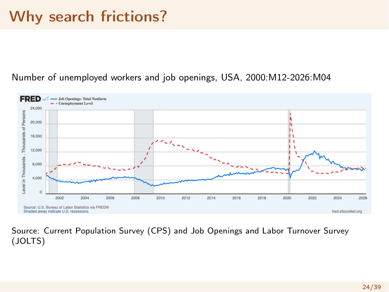 Unemployed workers and job openings, US, 2000–2026 (CPS + JOLTS). The simultaneous existence of both is the empirical fingerprint of search frictions.
The Stocks-and-Flows View
The labor market is not static: every month there are large gross flows between all three states, even when the stocks (, , ) barely move. Average US monthly flows (2000–2019) as a share of the source stock:
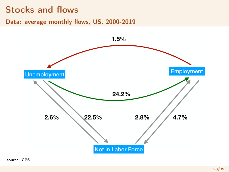 Average monthly transition rates between Employment, Unemployment, and Not-in-Labor-Force (US, 2000–2019, CPS). Note how much churn sits behind a "stable" unemployment rate — e.g. 24.2% of the unemployed find work each month, but flows in and out of NLF are just as large.
The big lesson of gross flowsA flat unemployment rate is not a quiet labor market. Millions transition every month; the stock is constant only because inflows ≈ outflows. This is why modern models focus on the rates of transition, not the levels.
A Descriptive Two-State Model of Unemployment
To get tractable, focus on E and U only (ignore NLF) and assume everyone is in the labor force, so . Define two transition probabilities:
- ==Separation / job-destruction rate == — probability an employed worker moves .
- ==Job-finding rate == — probability an unemployed worker moves .
graph LR
    E[Employed E] -->|separation rate d| U[Unemployed U]
    U -->|job-finding rate f| E
    class E,U internal-link;
Laws of Motion
Steady-State Unemployment
A ==steady state== has constant stocks () — workers still transition, but inflows equal outflows. Set and use :
The cleanest derivation is the flow-balance condition: inflow to = outflow from :
Solve for :
Reading the steady-state formulaUnemployment rises with the separation rate (more people losing jobs) and falls with the job-finding rate (faster re-employment). A labor market with lots of churn but fast matching ( and both high) can have low unemployment; a "sclerotic" market (low , low ) can have high long-term unemployment with few layoffs. The level of unemployment is about the ratio of the two rates, not either alone.
Why This Decomposition Is Useful
Data on and let us ask which margin drives unemployment:
- Is recession unemployment high because of high (a wave of layoffs) or low (people can't find work)? — both matter, but their relative roles changed across episodes (Shimer 2012).
- Do cross-country differences in unemployment come from or ?
- Why is youth unemployment so high — high , low , or both?
Empirical Patterns in and
Unemployment by Age (US, CPS 1976–2012)
| Age group | 20–24 | 25–34 | 35–44 | 45–54 | 55–64 |
|---|---|---|---|---|---|
| Avg unemployment rate (%) | 10.45 | 6.37 | 4.81 | 4.22 | 4.01 |
| Relative to 45–54 | 2.48× | 1.51× | 1.14× | 1 | 0.95 |
Unemployment falls monotonically with age — 20–24-year-olds face ~2.5× the rate of 45–54-year-olds.
Is it or ? (transition rates by age, "direct" flow approach)
| Age group | 20–24 | 25–34 | 35–44 | 45–54 | 55–64 |
|---|---|---|---|---|---|
| Job-finding (%) | 28.46 | 26.58 | 25.50 | 23.77 | 21.35 |
| Separation (%) | 2.62 | 1.51 | 1.13 | 0.96 | 0.84 |
A subtle but important pointThe job-finding rate actually falls with age — taken alone, that would predict unemployment rising with age (the opposite of what we see!). The resolution is the separation rate: for the young is ~2.7× that of prime-age workers, and this dominates. Young workers churn more (they're in lower-quality, less-stable matches), and that high is what drives their high unemployment. You cannot read off the cause from the unemployment rate alone — you need the flows.
Unemployment by Education (US men 25+, 1996–2014)
| < High school | High-school grad | Some college | College+ | |
|---|---|---|---|---|
| Population share (%) | 11 | 31 | 26 | 32 |
| Unemployment rate (%) | 8.7 | 6.1 | 4.8 | 2.8 |
| Separation (%) | 3.6 | 2.1 | 1.6 | 0.8 |
| Job-finding (%) | 50 | 45 | 45 | 39 |
Again the gradient in unemployment is driven mainly by separation rates (which fall sharply with education), not job-finding.
and Over Time
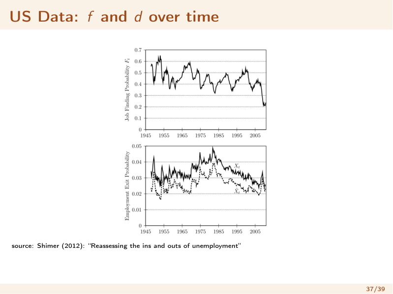 US job-finding and separation rates over time (Shimer 2012). Both are strongly cyclical — the relative contribution of "ins" (separations) vs. "outs" (finding) to unemployment fluctuations is itself a research question.
What's Still Missing
This toy model is deliberately incomplete. Open extensions:
- The labor-force participation decision (the margin we dropped) — quantitatively huge.
- Other states: part-time work, unpaid leave.
- Why are and what they are? Does it matter if separations are layoffs vs. quits (e.g. "the Great Resignation")? We need them to be endogenous equilibrium objects.
The destination: search-and-matchingThe Diamond–Mortensen–Pissarides (DMP) search-and-matching model takes frictions seriously and delivers (and sometimes ) as equilibrium outcomes, so unemployment arises endogenously. It became the workhorse of macro-labor (Nobel Prize 2010). Like any model it has limits, but it is the natural next step from this descriptive framework.
Summary
- Labor-market aggregates come from surveys (CPS households, CES establishments) and depend on definitions — the active-search requirement for is what the frictionless model lacks.
- Three states: E, U, NLF. Watch all three measures — , EPOP, participation — because workers exiting to mechanically lower the unemployment rate without any real improvement.
- Three sources of unemployment: sticky wages (only bites if rigid above equilibrium), structural (reallocation/mismatch), frictional (search & matching takes time; proven by coexisting vacancies and unemployment).
- The labor market has huge gross flows behind stable stocks — model the rates, not the levels.
- Two-state model: steady-state — unemployment rises with separations , falls with job-finding .
- Empirically, the age and education gradients in unemployment are driven mainly by separation rates , not job-finding — a fact invisible without flow data.
- Next step: DMP search-and-matching makes and endogenous and generates equilibrium unemployment.
Related Notes
- Built on: Lec_07-Labor Market — the frictionless model this lecture extends; supply, demand,
- Companion: Lec_09-Inequality & Polarization — heterogeneity across skill/occupation; which workers face high
- Built on: Lec_06-Equilibrium in the Goods Market — the general-equilibrium frame
- Future: Search and Matching Model — DMP; endogenous , , and equilibrium unemployment
- Concept: Sticky Wages, Frictional Unemployment, Stocks and Flows Model