
Fiscal Policy — Government Expenditure & Taxes
- #macroeconomics
- #fiscal-policy
- #government-spending
- #taxes
- #ricardian-equivalence
- #government-budget-constraint
- #public-debt
- #debt-dynamics
Fiscal Policy — Government Expenditure & Taxes
Part of: Macro-Economics Lecture 10 — Macro-Economics, "Fiscal Policy: Government Expenditure and Taxes" Key concepts: Government Budget Constraint, Ricardian Equivalence, Lump Sum Tax, Labor Income Tax, Consumption Tax, Crowding Out, Public Debt Dynamics, Primary Deficit
Where This Fits
We now put the government into the models already built: the two-period consumption model (Lec_02-Consumption and Saving), the goods market (Lec_06-Equilibrium in the Goods Market), and the labor market (Lec_07-Labor Market). The questions: how do government spending and taxes affect consumption, the interest rate, employment, and output — and when does the financing method (taxes vs. debt) matter?
Three modelling caveats stated upfront
- The model takes a deliberately negative view of government spending — this is an assumption, not a law. here is a pure resource drain (no productive public goods).
- The model is real — there is no inflation, which would change some results.
- Other fiscal tools (unemployment insurance, transfers beyond lump sums) are not covered.
Definitions
| Term | Reality | In the model |
|---|---|---|
| Government expenditure | Defense, education, health, municipal, development, debt repayment | Goods-market purchases + debt repayment |
| Government revenue | Labor/capital/corporate income tax, VAT, plus bond issuance | Lump-sum taxes (later: , ) + new debt |
| ==Budget deficit== | Expenditure − revenue in a period | Primary deficit |
| ==Government debt== | Stock of debt owed to domestic & foreign households | Stock (domestic only) |
The Government Budget Constraint
In each period, uses = resources:
Collapsing to a Lifetime Constraint
For two periods (0 and 1), assume no initial debt () and no debt left at the end (). Substituting period 1 into period 0:
The single most important fiscal identityThe present value of lifetime government spending equals the present value of lifetime tax revenue. Debt is only a device for moving taxes through time — it is not an extra source of resources. Every dollar of is ultimately paid for by some household's taxes, now or later.
Fiscal Policy in the Consumption Model
The two-period consumer with disposable income :
Substitute the government's lifetime constraint ():
The key substitutionIn the consumer's lifetime budget, taxes drop out and are replaced by spending . Only the present value of lowers the consumer's lifetime resources (PVLR). Bonds and the timing of taxes never appear.
Ricardian Equivalence
This identity delivers ==Ricardian Equivalence (RE)==:
graph TD
    A["Change T only (G fixed)"] --> B["PV of taxes unchanged<br/>(gov't constraint binds)"]
    B --> C["Consumer PVLR unchanged"]
    C --> D["Optimal consumption plan UNCHANGED"]
    E["Change G"] --> F["Consumer PVLR falls by PV(G)"]
    F --> G["Consumption plan DOES change"]
    class A,E internal-link;
Ricardian Equivalence — two statements
- Financing a given with taxes is equivalent to financing it with debt (same effect on consumers).
- A change in not accompanied by a change in does not affect PVLR or consumption. Intuition: a tax cut today with unchanged means the government borrows; rational consumers know they will repay it via higher future taxes, so they save the entire tax cut to meet that future liability.
When RE Fails (Realistically, It Does)
Reasons RE breaks down
- Different planning horizons for government vs. consumers (finite lives, no bequest motive).
- Heterogeneity in horizons (young vs. old).
- Credit-market imperfections: government borrows cheaper than households; borrowing-constrained consumers can't smooth.
- Uncertainty and information frictions.
- Distortionary (non-lump-sum) taxes and elastic labor supply.
- Inflation (the model assumes none).
Goods-Market Effects
Example 1 — Lower and Lower (balanced)
Government cuts and cuts taxes by the same amount.
- For consumers this is a positive income shock (PVLR rises because PV(G) falls) → they consume more and save more, but smooth, so .
- The saving curve shifts right → lower , more investment .
- GDP is unchanged (no change in ): the rise in exactly offsets the fall in .
This is the mirror image of crowding out (see Lec_06-Equilibrium in the Goods Market).
graph LR
    A["G ↓ and T ↓ (equal)"] --> B["PVLR ↑ → C ↑, S ↑"]
    B --> C["S curve shifts RIGHT"]
    C --> D["r ↓, I ↑, Y unchanged"]
Example 2 — Same , Lower , RE Fails
- If RE holds: no response at all.
- If RE fails: consumers treat the tax cut as a positive income shock → ↑, private ↑, but government saves less (borrows more).
- Net national saving falls (since ↑, and unchanged) → S curve shifts left → ↑, ↓. This is crowding out via deficit-financed tax cuts.
Empirical Evidence on the Timing of Taxes
Shapiro & Slemrod (1995) — the 1992 withholding change
In Jan 1992, President Bush reduced tax withholding (not tax rates) — a pure timing shift (~$29/worker/month, ~$25bn total), deferring payment ~1 year with no change in total obligation. Pure Ricardian logic says: save it all.
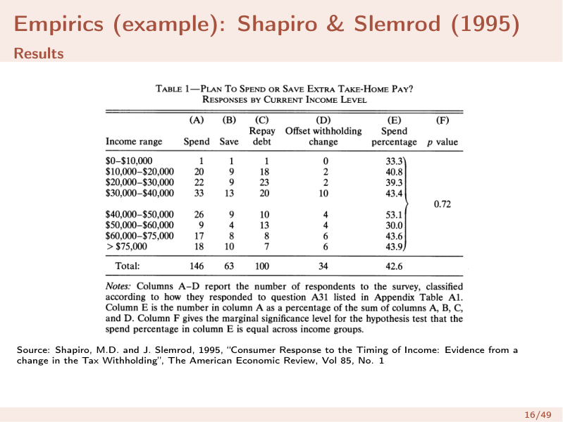 Survey responses by income group (Shapiro & Slemrod 1995). ~43% of households planned to spend the extra take-home pay (s.e. ≈ 3pp).
What the 43% rules outThe estimate that ~43% planned to spend is strong evidence against both extremes: it is far from 0% (the pure life-cycle / Ricardian prediction) and far from ~100% (the naive Keynesian consumption function). Reality sits in between — and no clean relationship with liquidity constraints (income, financial condition) emerges. Consumers behave neither fully rationally-forward-looking nor mechanically Keynesian.
Stimulus Payments (transfers, not timing shifts)
Governments use direct transfers in crises (2008 financial crisis; Covid-19). Key questions: what is the implied MPC? and is this the most efficient stimulus?
- Shapiro & Slemrod (2009) — 2008 US rebates ($300–600/person, ~130m households, >$100bn). Survey of intended use; notably no difference between those who had already received vs. not.
- Feldman & Heffetz (2022) — Israel mid-2020 grant (NIS 750/adult, less per child, ~NIS 6.5bn ≈ 0.5% of GDP). Substantial donate/help categories; results broadly in line with US data.
The policy trade-offStimulus transfers are easy to implement but expensive and untargeted. ~40% of Israeli respondents said they were not hurt by Covid — so broad transfers partly pay people who don't need to spend. Open questions: can we target likely spenders? what is the opportunity cost of the budget? does timing (early vs. late crisis) matter? is Covid special (people couldn't spend)?
Fiscal Policy in the Labor Market Model
Add three taxes to the household budget constraint — lump-sum , labor-income tax , consumption tax :
Solving (Lagrangian)
Divide the second by the first:
This is the static FOC with taxes. The marginal benefit of working is the wage net of income tax, converted into consumption net of consumption tax. Both and work the same way — they shrink the effective return to labor.
Lump-Sum Tax → Pure Income Effect
enters exactly like a (negative) wealth term :
| Change | Effect on worker | Labor supply |
|---|---|---|
| ↑ (more taxes / lower transfers) | Income falls → work more | shifts right |
| ↓ (lower taxes / more transfers) | Income rises → work less | shifts left |
Distortionary Tax ( or ) → Income and Substitution Effects
A labor-income tax rotates the budget line in (Leisure, ) space: the slope flattens from to .
graph TD
    A["τ_N ↑ : after-tax wage (1-τ_N)w falls"] --> B["Substitution effect: leisure cheaper → work LESS"]
    A --> C["Income effect: poorer at any N → work MORE"]
    B --> D["Net: if SE dominates (our assumption) → work LESS<br/>N^S shifts LEFT"]
    C --> D
Consistency with the upward-sloping supply curveIn Lec_07-Labor Market we assumed the substitution effect dominates so that slopes up. The same assumption implies a higher labor-income tax lowers labor supply (shifts left). A distortionary tax therefore does shift the supply curve, unlike a lump-sum tax which moves it via the income effect only. Permanent tax changes also hit PVLR substantially.
Worked Example — ↑ financed by lump-sum ↑ (short run)
| Question | Answer |
|---|---|
| Does shift? | No — unchanged |
| Does shift? | Yes — negative income effect → shifts right |
| New labor-market eqm | More , lower |
| New goods-market eqm | Consumers smooth, $ |
| Output, , , | ↑, but , , ↓, ↑. Note |
type: macro-shocks
figure: fiscalWorked Example — Permanent ↑ with PVLR held fixed (long run)
Proceeds rebated so PVLR is unchanged → neutralizes the income effect, leaving only substitution/distortion.
- Short run: no shift; shifts left (distortion) → lower , higher .
- Long run: lower expected future labor → firms cut optimal future capital → lower investment today → shifts left (less ) → lower and lower relative to the short run (ambiguous vs. the initial state).
Why distortionary taxes are costlier than lump-sumLump-sum taxes are non-distortionary — they only move the income effect. Distortionary taxes (, ) drive a wedge between the worker's and firm's valuation of labor, shrinking employment even before any income effect, and depressing long-run capital. This is the efficiency cost ("deadweight loss") of realistic taxation.
Dynamics of Public Debt
Debt and deficits dominate policy debate because the government must keep debt at sustainable levels to keep borrowing at reasonable rates (else default risk). Debt is tracked as a ratio to GDP, so strong GDP growth makes more debt sustainable.
Illustrative assumptionsGrowth rate and interest rate are exogenous and constant; no inflation.
Deriving the Law of Motion
Start from the budget constraint with primary deficit :
Use lower-case for GDP ratios (, ) and constant growth (so ). Dividing through:
Subtracting gives the change in the debt ratio:
The two forces on the debt ratioThe debt-to-GDP ratio rises with (1) the primary deficit and (2) the interest-growth differential . If , debt service outpaces growth and the existing stock keeps pushing the ratio up — even with a balanced primary budget. If , growth erodes the ratio.
Calculating the Path
One-period projectionWith , , primary deficit , current :
Steady-State (Constant) Debt Ratio
Set :
Steady-state debt ratioWith , , : . If the steady-state can be negative (sustainable only as net assets).
Stability
graph TD
    A["Found a steady state b*"] --> B{"Is r < g?"}
    B -->|Yes| C["b converges to b*<br/>(STABLE)"]
    B -->|No, r > g| D["b diverges from b*<br/>(UNSTABLE)"]
    class C internal-link;
    class D internal-link;
The stability condition is
- (growth beats interest): any deviation in converges back to steady state — debt is self-correcting.
- (interest beats growth): deviations diverge — debt dynamics are explosive, and a high-debt country can spiral. This is the crux of every debt-sustainability debate.
Solving for Required Growth
Rearranging for :
Required growth to stabilize debtWith , , : — a very high growth rate needed to sustain that deficit.
Summary
- Government budget constraint: ; in PV terms, PV(spending) = PV(taxes). Debt only moves taxes through time.
- In the consumer's lifetime budget, taxes are replaced by — only PV() lowers PVLR.
- Ricardian Equivalence: changing alone (with fixed) doesn't affect consumption; tax vs. debt financing are equivalent. Fails in reality (finite horizons, credit constraints, distortionary taxes, uncertainty, inflation).
- Goods market: balanced ↓/↓ → ↑, ↑, ↓, unchanged (reverse crowding out). Deficit-financed ↓ with RE-failure → ↑, national ↓, ↑, ↓.
- Evidence: ~43% spend a tax-timing windfall (Shapiro–Slemrod) — between Ricardian (0%) and Keynesian (~100%). Stimulus transfers are easy but untargeted.
- Labor market with taxes: static FOC becomes . Lump-sum = pure income effect ( right when ↑); distortionary add a substitution effect → shifts left, with long-run capital decline.
- Debt dynamics: . Steady state . Stable iff ; if debt diverges.
Related Notes
- Built on: Lec_02-Consumption and Saving — two-period model, Euler equation, PVLR (the engine of Ricardian Equivalence)
- Built on: Lec_06-Equilibrium in the Goods Market — , real interest rate, crowding out (this lecture is the mirror image)
- Built on: Lec_07-Labor Market — static FOC, income vs. substitution effects (extended here with taxes)
- Companion: Lec_09-Inequality & Polarization — distributional analysis where heterogeneity makes fiscal policy bite differently
- Concept: Ricardian Equivalence, Government Budget Constraint, Public Debt Dynamics, Lump Sum Tax, Labor Income Tax