
Production
- #macroeconomics
- #production-function
- #cobb-douglas
- #tfp
- #marginal-products
- #development-accounting
- #growth-accounting
Production
Part of: Macro-Economics Lecture 04 — Macro-Economics Key concepts: Production Function, Total Factor Productivity, Cobb-Douglas, Marginal Product of Labor, Marginal Product of Capital, Development Accounting, Solow Residual
Where This Fits in the Big Picture
The course is building toward a full model of the economy. The national accounts identity tells us:
- We already have a theory of consumption () from Lec 02.
- This lecture gives us the supply side: a model of how is produced.
- The production model will later be used to derive:
- Demand for investment (Lec 05)
- Demand for labor (Lec 07)
- The foundation for growth models (later in course)
The Production Function
Basic Setup
To model production we ask: what are the inputs, and how do they combine to make output?
We focus on two inputs:
- ==Capital ()== — machines, buildings, equipment
- ==Labor ()== — total hours of work
We also include a third "input" that is not a physical thing: ==Total Factor Productivity ()==, which captures how efficiently and are used. reflects technology, management quality, efficient resource allocation, human capital, and institutions.
The production function is:
- = aggregate real output (GDP) in period
- = capital stock in period
- = labor input (total hours) in period
- = Total Factor Productivity in period
- = a time-invariant function (the inputs change, not the function itself)
Why only K and N?In reality, economies use energy, land, raw materials, and more. We focus on and because they account for most income (wages + capital returns ≈ entire GDP under competitive markets) and because data is available to measure them.
Marginal Products
The ==marginal product== of an input is the extra output you get from adding one more unit of that input, holding everything else constant.
In data these can be approximated as:
Why marginal products matterMarginal products determine factor prices in competitive markets. The wage a firm pays equals MPN; the rental rate for capital equals MPK. This is the central pricing result we'll use throughout the course.
Four Key Properties of the Production Function
These four assumptions hold throughout the entire course. They are what makes the production function economically sensible.
Property 1 — Positive Marginal Products
More input → more output. Adding workers or machines always produces something extra (though perhaps less and less).
Property 2 — Diminishing Marginal Products
The last unit of an input contributes less than the one before it. Intuitively: if you keep adding workers to a factory with a fixed number of machines, eventually they start getting in each other's way.
Graphically: the vs curve slopes upward (Property 1) but gets flatter as grows (Property 2). The slope of the curve is the marginal product.
type: production-capital
figure: productionProperty 3 — Complementarity
More workers make capital more productive, and more capital makes workers more productive. Intuition: a construction worker with a digger (capital) is far more productive than one with a spade.
Why complementarity mattersComplementarity creates a force toward a balanced mix of capital and labor. It also means that in the long run, when firms accumulate more capital, labor demand rises — this is key for Lec 07's long-run analysis.
Property 4 — Constant Returns to Scale (CRS)
If you multiply both inputs by the same factor , output scales by exactly :
Double the factory and the workforce → exactly double the output. Neither economies nor diseconomies of scale.
Why CRS?Two pieces of empirical evidence:
- Balanced growth: economies grow over long periods without either the labor force or capital perpetually exploding.
- Stable factor shares: the share of GDP going to wages (vs. capital) has been remarkably stable over time across countries — this is exactly what CRS predicts (see below).
Useful implication of CRS: only the ratio matters, not the levels. Setting :
So GDP per worker depends on capital per worker — the foundation of growth models.
Checking the Properties — Quick Examples
| Function | Prop 1 (+MPs) | Prop 2 (Dim.) | Prop 3 (Comp.) | Prop 4 (CRS) |
|---|---|---|---|---|
| ✅ | ❌ (constant MPs) | ❌ () | ✅ | |
| ✅ | ✅ | ✅ | ✅ () | |
| ✅ | ❌ (increasing MPs) | ❌ | ❌ |
The Cobb-Douglas Production Function
The most widely used functional form in macroeconomics:
For CRS we need , so .
Cobb-Douglas satisfies all four propertiesYou can verify: ; (since ); ; and with , doubling inputs doubles output.
Income Shares
In a competitive market, factors are paid their marginal products. The capital share of income is:
Similarly, the labor share equals .
Deriving the capital share
This is powerful: we can read the parameters directly from national accounts data. For most countries, empirical estimates give:
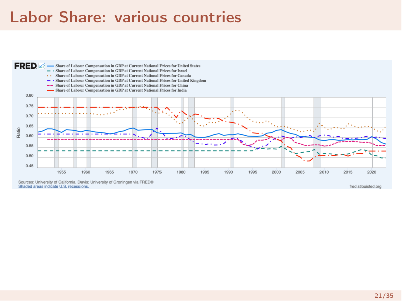 Labor share of income across countries. Its rough stability around ~0.6–0.7 is the empirical basis for treating as a constant and for the CRS assumption.
Elasticities
The ==elasticity== of output with respect to an input is the percentage change in output for a 1% change in that input:
For Cobb-Douglas, take logs:
Therefore:
So is both the capital income share and the capital elasticity of output — one of the reasons Cobb-Douglas is so useful.
The log-linearization trickTaking logs of the Cobb-Douglas production function converts it into a linear equation in log-variables. This is the standard technique used throughout growth accounting, empirical macro, and this course. Get comfortable with it.
Competitive Markets and Firm Optimization
Setup
Firms are price takers: they take output price (normalized), wage , and rental rate of capital as given. They maximize profits:
First-Order Conditions
Taking derivatives and setting to zero:
Factors are paid their marginal products. This is a central result used throughout the rest of the course.
Intuition for MPN = wIf MPN > w, the firm earns more from the last worker than it pays → hire more. If MPN < w, the last worker costs more than it produces → fire them. Profit-maximisation drives you to MPN = w.
Development Accounting
What is it?
Development accounting uses the production model to understand why some countries are richer than others. It asks: how much of the income gap between countries can be explained by differences in and vs. differences in (TFP)?
Step 1 — Capital Only
Assume all countries have the same . Given data on capital per worker and the Cobb-Douglas form:
With , compare predicted to actual :
| Country | Observed | Predicted | Actual |
|---|---|---|---|
| USA | 1.00 | 1.00 | 1.00 |
| Switzerland | 1.56 | 1.16 | 1.20 |
| Italy | 1.35 | 1.11 | 0.65 |
| Japan | 0.90 | 0.96 | 0.63 |
| Israel | 0.65 | 0.86 | 0.62 |
| India | 0.12 | 0.49 | 0.11 |
| Ethiopia | 0.027 | 0.30 | 0.044 |
Conclusion: Capital differences alone predict much smaller income gaps than we actually observe (e.g., Italy has almost as much capital as Switzerland, yet half the income). There must be another factor — TFP.
Step 2 — Letting TFP Differ
Now back out the implied TFP for each country:
| Country | Actual | Predicted | Implied |
|---|---|---|---|
| USA | 1.00 | 1.00 | 1.00 |
| Italy | 0.65 | 1.11 | 0.585 |
| India | 0.11 | 0.49 | 0.224 |
| Ethiopia | 0.044 | 0.30 | 0.147 |
TFP gaps are large. For US vs India:
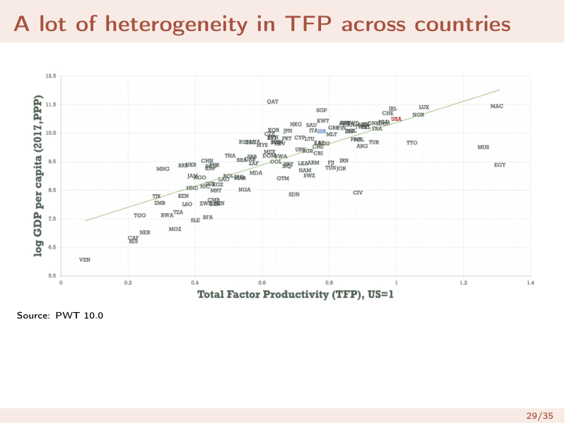 Large dispersion in implied TFP across countries (PWT). Since capital differences are far too small to explain observed income gaps, the residual — TFP — does most of the work.
Key findingTFP is responsible for more of the income gap than capital. This makes TFP simultaneously the most important variable in the model and the hardest to explain — it is sometimes called a "measure of our ignorance." Research tries to pin down TFP using R&D, education, governance, and institutions.
Growth Accounting and the Solow Residual
What is it?
Development accounting looks across countries at a point in time. ==Growth accounting== uses the same framework to decompose output growth over time within a single country into contributions from:
- Capital growth ()
- Labor growth ()
- TFP growth () — the Solow Residual
The Decomposition
Start from . Differentiating with respect to time and dividing by :
Rearranging for the Solow Residual:
Four-Step Procedure
- Collect data on , , (with quality adjustments if possible).
- Estimate elasticities and — for Cobb-Douglas these equal the income shares and , which we can read from national accounts.
- Calculate capital and labor contributions ( and ).
- Calculate TFP growth as a residual: everything unexplained by inputs.
Numerical example, , , ,
So 70% of growth is explained by TFP — capital and labor contributions are much smaller.
The Real Business Cycle connectionThe fact that TFP fluctuates significantly over time (not just across countries) motivates the Real Business Cycles literature, which argues that "productivity shocks" () are a key driver of economic fluctuations — booms happen when is high, recessions when falls.
Summary
- Production function is the supply side of the macro model. (TFP) captures everything that makes an economy more productive beyond raw inputs.
- Four key properties: positive MPs, diminishing MPs, complementarity, CRS. These are maintained throughout the course.
- Cobb-Douglas satisfies all four. Parameters and can be read from income share data.
- Competitive firm optimization: MPN = w and MPK = R — factors are paid their marginal products.
- Development accounting: capital differences alone can't explain cross-country income gaps; TFP differences are equally or more important.
- Growth accounting / Solow Residual: output growth = capital contribution + labor contribution + TFP growth. TFP is backed out as the residual.
Related Notes
- Predecessor: Lec_02-Consumption and Saving — completed the demand side
- Next: Lec_05-Investment — uses MPK from this model to derive investment demand
- Future: Lec_07-Labor Market — uses MPN from this model to derive labor demand
- Future: Growth Models — Cobb-Douglas + CRS is the foundation of the Solow model
- Problem Sets: Problem Set 3 — Cobb-Douglas properties, labor shares, TFP, growth accounting