
Consumption and Saving
- #macroeconomics
- #consumption
- #saving
- #euler-equation
- #life-cycle-hypothesis
- #permanent-income-hypothesis
- #intertemporal-choice
- #fisher-model
Consumption and Saving
Part of: Macro-Economics Key concepts: Euler Equation, Life-Cycle Hypothesis, Permanent Income Hypothesis, Intertemporal Choice, Consumption Smoothing, Borrowing Constraints
Why We Care — Stylised Facts
Consumption is ~67% of US GDP (FRED, 2025), and the single largest expenditure item in the national accounts. Understanding how households decide to consume vs. save is essential to understanding GDP, business cycles, and fiscal policy.
Components of private consumption
| Category | Lasts | Example |
|---|---|---|
| Durable goods | Long | Cars, appliances |
| Non-durable goods | Short | Food, clothing |
| Services | Intangible | Haircuts, cleaning |
Cyclical facts (US, 1947–2025)
- Aggregate : correlation with GDP ≈ 0.8; ~0.85× as volatile as GDP.
- Services : correlation 0.69; only 0.72× as volatile.
- Non-durables : correlation 0.66; 0.77× as volatile.
- Durables : correlation 0.58 but ~2.9× as volatile as GDP.
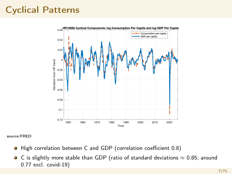 Cyclical components of consumption and GDP, USA. Consumption tracks GDP closely (corr ≈ 0.8) but is smoother — the visual signature of consumption smoothing.
Key puzzleConsumption is strongly correlated with income but not just a constant fraction of it. Households must be using savings to smooth consumption across periods. We need a theory of why and how they smooth.
The "Old" Keynesian Consumer
Definitions
- Marginal propensity to consume (MPC): — extra per extra .
- Average propensity to consume (APC): .
Keynesian consumption function
Assumption: MPC () is constant.
Predictions:
- Consumption is determined by current income.
- Saving rises with current income.
Why it fails
Under this model, consumption differences must be perfectly correlated with income differences:
In the data, that correlation is only 0.4–0.65 across categories. The model also:
- Ignores dependence on future income.
- Ignores the interest rate.
- Lacks micro-foundations.
What's missingWe need a model of inter-temporal choice and forward-looking behaviour — Fisher's two-period model.
Consumption, Saving, and Wealth
Household saving
where = saving (can be negative), = disposable income, = consumption.
Aggregate saving
Flow vs. stock
- Saving is a flow (per period).
- Wealth is a stock. Positive saving increases wealth.
Why Save or Borrow?
- Life-cycle — save for retirement.
- Life-cycle — borrow against future earnings (e.g. student loans).
- Precautionary — uncertain income → save against downside.
- Time discounting — preferences over today vs. tomorrow.
The Two-Period Model — Setup
Notation
| Exogenous | Endogenous |
|---|---|
| : current income | : current consumption |
| : future income | : future consumption |
| : initial assets | : next-period assets |
| : real interest rate | |
| : discount factor |
Preferences — three assumptions
- More is better: .
- Diminishing marginal utility: .
- Impatience: today's utility weighted more than tomorrow's via .
Plus the technical conditions and .
Objective — lifetime utility
Budget constraint — two equivalent forms
Sequential (flow):
Lifetime (PVLR):
where PVLR = Present Value of Lifetime Resources.
Why these are equivalentSolve the first-period constraint for , substitute into the second, divide by . The sequential form shows cash flows each period; the lifetime form shows the single lifetime budget line.
The Euler Equation
Setting up the Lagrangian
FOCs give and . Combining:
This is the Euler equation — a necessary condition for an optimal consumption plan.
Interpretation
Consider saving more today:
- Cost: lose in utility now.
- Benefit: gain in utility tomorrow.
At the optimum the two are equal. If they're not, reallocate until they are.
Consumption-saving trade-off
| Condition | Implication |
|---|---|
| (perfect smoothing) — the market rate just offsets impatience | |
| — market over-compensates for impatience → save | |
| — impatience dominates → borrow / front-load |
General (T-period) form
Graphical Picture
- Budget line in space: slope , passes through the endowment .
- Indifference curves: convex, slope = MRS.
- Optimum: tangency where — exactly the Euler equation.
type: consumption-choice
figure: two-periodJensen meets economicsA concave utility function means the utility of the average exceeds the average of the utilities — i.e. smoothed consumption is preferred to volatile consumption with the same mean. This is the mathematical core of the consumption-smoothing motive.
Comparative Statics
The discount factor
Higher ⇒ more patient ⇒ must rise ⇒ lower , higher (save more).
appears in the Euler equation but not the budget constraint — a pure preference shift.
The interest rate — the ambiguous case
affects both the budget constraint (via PVLR) and the Euler equation. Two effects:
| Effect | Direction |
|---|---|
| Substitution effect — current gets relatively more expensive | |
| Income effect (borrower) — PVLR falls | |
| Income effect (lender) — PVLR rises |
Course conventionFor a borrower, substitution and income effects both push down — unambiguous. For a lender, they oppose — ambiguous. Unless told otherwise, assume .
Generalisation to Periods
PVLR:
Budget:
Utility:
Euler:
The Life-Cycle Hypothesis (Modigliani)
Stylised setup
Assume , , , constant income for working periods, zero income for retirement periods.
Because , the Euler equation gives perfect smoothing: for all .
PVLR , and with :
Implications:
| Phase | Income | Consumption | Saving |
|---|---|---|---|
| Working () | |||
| Retirement () |
type: consumption-choice
figure: lifecycleWealth profile: rises during working years, peaks at retirement, then depletes toward zero at death. This hump-shape is seen clearly in Survey of Consumer Finances (US), StatCan, and IFS (UK) data.
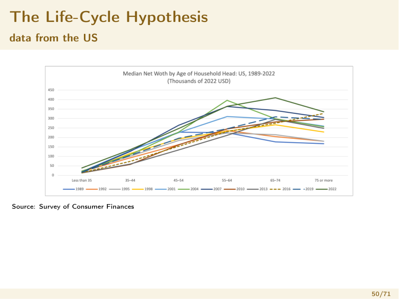 Hump-shaped wealth by age, US Survey of Consumer Finances — wealth accumulates through working life, peaks near retirement, then is drawn down, exactly as the LCH predicts.
Consumption vs. expenditure
Banks, Blundell & Tanner (1998) found a "retirement-savings puzzle": expenditure drops sharply at retirement. Aguiar & Hurst (2005) resolved this — what falls is work-related expenditure (food spending, clothing) while time spent on home production rises to substitute. True consumption stays smooth.
Expenditure ≠ consumptionWhen households retire they buy fewer prepared meals and more raw ingredients and cook themselves. Measured spending falls but welfare-relevant consumption is roughly flat — as the LCH predicts.
The Permanent Income Hypothesis (Friedman)
Permanent income : the hypothetical constant income stream that has the same PVLR as the actual (variable) income stream.
Core claimConsumption depends on permanent income (i.e., PVLR), not current income alone.
Predictions for income shocks
| Shock type | Expected? | today | today |
|---|---|---|---|
| Expected rise in | Yes | 0 | (whole rise saved until realised) |
| Unexpected temporary rise in | No | Small (split over periods) | (most of shock saved) |
| Unexpected permanent rise in | No | (full MPC ≈ 1) | 0 |
| Unexpected future rise in | No | (borrow against it) |
Key subtletyConsumption re-optimises when new information arrives, not when the income change actually happens. An anticipated raise has already been priced into today's consumption — no smoothing response when it arrives.
Worked example (two periods, )
Optimal plan: .
For a shock to income:
| Shock | Change in today |
|---|---|
| One-off in period 0 | |
| One-off in period 1 | |
| Permanent | (full pass-through) |
Log-utility example,
With , Euler gives , and substituting:
Excess Sensitivity and Borrowing Constraints
The puzzle
Micro-data studies find consumption is too sensitive to current-income changes relative to the PIH benchmark.
Candidate explanations
- "Rule of thumb" consumers — a fraction just spend current income.
- Myopia / short horizons.
- Consumption vs. expenditure measurement issues.
- Borrowing constraints — can't borrow to smooth.
Borrowing constraint mechanics
If the household wants to borrow but can't, the Euler equation becomes:
Current consumption is below the unconstrained optimum. Extra income today goes straight into consumption (high MPC) until the constraint no longer binds.
type: consumption-choice
figure: borrowingPolicy relevanceBorrowing-constrained households respond strongly to temporary fiscal transfers — this is why stimulus checks work even though PIH says they shouldn't. Targeting transfers to the constrained maximises stimulus per dollar.
"Wealthy hand-to-mouth" (Kaplan & Violante, 2014)
Not just the poor. Roughly 20% of US households have illiquid assets (housing, retirement accounts) but little liquid wealth — they behave as hand-to-mouth despite being rich. In France, Germany, Italy and Spain, the wealthy HtM outnumber the poor HtM by 3-to-1.
Implications:
- Borrowing frictions ≠ poverty.
- The MPC out of transitory income shocks can be high even in non-poor households.
- Fiscal multipliers depend on the share of HtM consumers in the economy.
Summary — What This Lecture Teaches
- Stylised facts: is large, correlated with , and smoother than (except durables).
- Old Keynesian is too simple — no role for future income, interest rates, or micro-foundations.
- Inter-temporal optimisation delivers the Euler equation — the central equation of consumption theory.
- Life-cycle hypothesis: save during working years, dissave in retirement → hump-shaped wealth profile (confirmed in data).
- Permanent income hypothesis: consumption tracks PVLR; anticipated income changes don't move ; information arrival does.
- has ambiguous effects — substitution vs. income. Convention: .
- Borrowing constraints explain excess sensitivity and give fiscal policy a transmission channel — relevant for the wealthy-HtM population, not just the poor.
Related Notes
- Foundational: Intertemporal Choice, Present Value, Utility Maximisation
- Companion: Lec_01-Data Review — stylised macro facts
- Future applications: Fiscal Policy, Ricardian Equivalence, New Keynesian Models
- Key references in lecture: Banks, Blundell & Tanner (1998); Aguiar & Hurst (2005); Kaplan & Violante (2014)