
Franchise FCF NPV, NPV vs IRR, Loan Effective Rate, Amortisation & Growing Cash Flows (2025 Moed B)
- #financial-management
- #fundamentals-of-finance
- #past-paper
- #worked-solution
- #free-cash-flow
- #npv
- #irr
- #effective-rate
- #loans
- #amortization
- #growing-annuity
Franchise FCF NPV, NPV vs IRR, Loan Effective Rate, Amortisation & Growing Cash Flows (2025 Moed B)
Part of: Financial Management Fundamentals of Finance, Moed B (2025). Open-ended calculation questions, no multiple choice. Builds on: Lesson_06-Capital Budgeting & Free Cash Flow, Lesson_02-Perpetuities, NPV & IRR, Lesson_03-Rate Conversion, Effective Rates & EAC, Lesson_05-The Four Loan Types, Lesson_01-Time Value of Money Practice: HW_07-Free Cash Flow & Project NPV, HW_02-NPV, IRR & Project Choice, HW_04-Effective Interest Rates, HW_06-Loans & Amortization
Whole paper reconstructed, no official keyThe question paper for this sitting is not on disk. The only source is a student's Excel workbook (
2025B.xlsx) with short labels, inputs and formulas. Every question below is reconstructed from those cells, and every answer is AI-written, re-derived from the reconstructed question. The workbook is a student's own working, not an official solution. Check each question wording against the real paper before relying on any of it.
Question numberingOnly the sheet
Question 1is clearly Q1. The other four tabs are named1,2,Sheet4and7. Two tabs cannot both be "question 1", and nothing in the cells says2and7are question numbers 2 and 7, so I numbered them in sheet order and show the tab name in each heading.
This note Workbook sheet Topic Q1 Question 1Franchise project: free cash flow and NPV Q2 1Projects A, B, C: NPV and IRR Q3 2Loan with fees: effective annual rate Q4 Sheet4Equal-payment loan and amortisation table Q5 7Growing outflows against periodic inflows: NPV
AI-solved questionsQ1, Q2, Q3, Q4, Q5 are all AI-solved from the workbook. Q1 also corrects a workbook error (the
NPVfunction), see below.
What this paper tests
| Question | Core idea | Where it is taught |
|---|---|---|
| Q1 | Build Free Cash Flow with Depreciation tax shield, Working Capital and tax on losses, then Net Present Value | Lesson_06-Capital Budgeting & Free Cash Flow, HW_07-Free Cash Flow & Project NPV |
| Q2 | Net Present Value and Internal Rate of Return of three projects; ranking conflict, NPV Profile | Lesson_02-Perpetuities, NPV & IRR, HW_02-NPV, IRR & Project Choice |
| Q3 | All-in cost of a loan with fees: IRR of the borrower's cash flows, then Rate Conversion to an Effective Interest Rate | Lesson_03-Rate Conversion, Effective Rates & EAC, HW_04-Effective Interest Rates |
| Q4 | Equal-payment Mortgage: PMT, Amortization table, Outstanding Balance | Lesson_05-The Four Loan Types, HW_06-Loans & Amortization |
| Q5 | Irregular cash flows with a Growing Annuity of costs, discounted to NPV | Lesson_01-Time Value of Money, Lesson_02-Perpetuities, NPV & IRR |
Intuition: the one move behind each question
- Q1: discount cash, not profit. Subtract depreciation for tax, add it back, and treat working capital as cash tied up and later released.
- Q2: NPV says how much value a project adds; IRR is the discount rate at which it adds nothing. They can rank projects differently.
- Q3: the real cost of a loan is the IRR of what you actually receive and pay, fees included. Fees raise it above the stated rate.
- Q4: each payment is fixed; interest is rate times opening balance and the rest repays principal.
- Q5: lay the cash flows on a timeline, net them year by year, discount. Excel's
NPVstarts at .
Q1 — Franchise project: free cash flow and NPV (sheet Question 1)
Reconstructed question: the question paper is not on disk. This wording was inferred from the worked spreadsheet; check it against the real paper.
A company is considering buying a franchise (cost 10,000 at , depreciated straight-line over 2 years, so 5,000 per year) to sell devices alongside its screens. The discount rate is and the tax rate is 20%. Units in the workbook are not stated beyond a "(thousand)" label next to the purchase price.
| Year 1 | Year 2 | Year 3 | |
|---|---|---|---|
| Expected device sales (units) | 9,000 | 7,000 | 14,000 |
| Devices purchased (units) | 15,000 | 5,000 | 10,000 |
Purchase price per device 2, sales price per device 3. Further information:
- Inventory holding cost is 0.15 per unit, charged on inventory balances of 6,000 units at and 4,000 units at (as entered in the workbook).
- Each year, 25% of expected device sales are lost screen sales; the expected loss (in thousands) equals 25% of the expected device sales.
- Working capital at the start of each year: inventory = 1/3 of that year's cost of purchases, receivables = 30% of that year's sales, suppliers (payables) = 10% of that year's cost of purchases. Working capital is fully recovered at the end of year 3.
- Taxes are symmetric: a negative EBIT gives a tax saving.
a. Compute the free cash flow for . b. Compute the NPV and decide whether to buy the franchise.
AI-written answer, not official. Check before relying on it.
a. Free cash flow
Use the FCF build from Lesson_06-Capital Budgeting & Free Cash Flow:
Step 1: revenue and costs. Sales units: 27,000, 21,000, 42,000. The "cost of goods sold" row is the cost of purchases units bought: 30,000, 10,000, 20,000 (the workbook expenses purchases as they are made). Lost screen sales: 2,250, 1,750, 3,500.
Step 2: working capital (balance at the start of each year, from that year's flows):
| (for year 1) | (for year 2) | (for year 3) | ||
|---|---|---|---|---|
| Inventory purchases | 10,000 | 3,333.33 | 6,666.67 | 0 |
| Receivables sales | 8,100 | 6,300 | 12,600 | 0 |
| Suppliers purchases | 3,000 | 1,000 | 2,000 | 0 |
| Working capital | 15,100 | 8,633.33 | 17,266.67 | 0 |
| Cash flow from WC (opening minus closing) |
Step 3: the FCF table.
| Sales | 27,000 | 21,000 | 42,000 | |
| Cost of purchases | ||||
| Gross profit | 11,000 | 22,000 | ||
| Inventory holding cost | ||||
| Lost screen sales | ||||
| Depreciation | ||||
| EBIT | 4,250 | 18,500 | ||
| Tax at 20% (negative EBIT gives a saving) | ||||
| NOPAT | 3,400 | 14,800 | ||
| Add back depreciation | ||||
| Cash flow from working capital | ||||
| Franchise acquisition (CAPEX) | ||||
| Free cash flow | 2,786.67 | 32,066.67 |
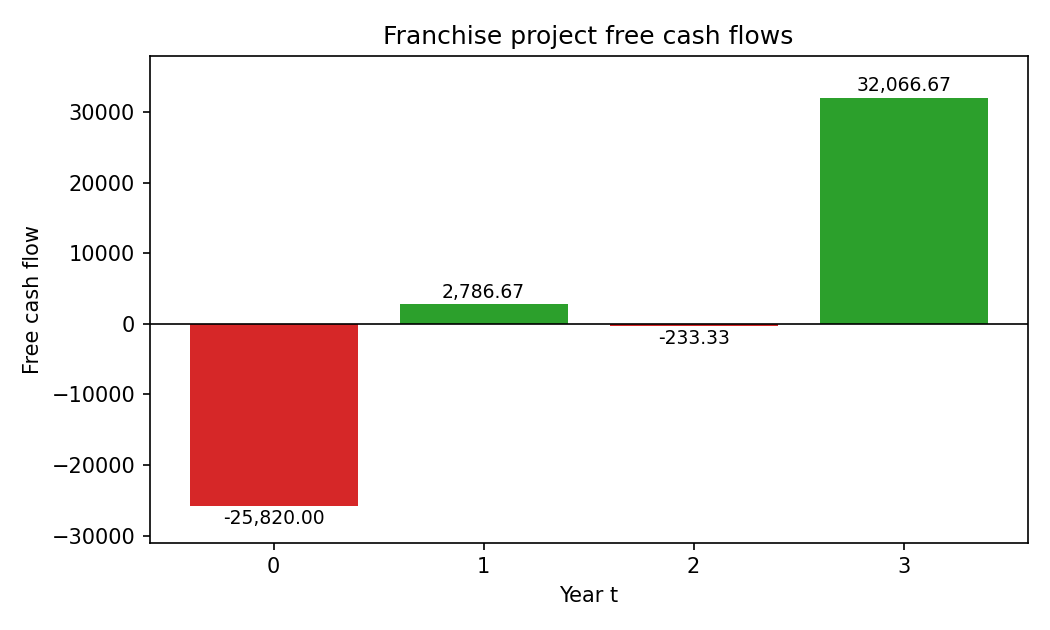
Holding cost: and . Depreciation: in years 1 and 2.
b. NPV and decision
Discount each flow by , with not discounted:
| FCF | ||
|---|---|---|
| 0 | ||
| 1 | 2,786.67 | 2,604.36 |
| 2 | ||
| 3 | 32,066.67 | 26,175.95 |
In Excel: =C18 + NPV(C2, D18:F18), the flow added outside the function (see Lesson_02-Perpetuities, NPV & IRR).
Decision: on the workbook's figure for lost screen sales, , so the franchise adds value and should be bought. Check point 1 below: a larger loss per sale reverses this.
Workbook value differs: 2,576.18 is not the NPV atThe workbook computes
=NPV(C2, C18:F18). Excel'sNPVtreats the first value as , so it discounts the flow of by one period too many. The result is the NPV one year early: . The correct NPV at is 2,756.51. The decision (invest) is unchanged. (Sheet1and sheet7use the function correctly.)
The#N/Ain cell G17Column G in this sheet is a set of annotation cells:
="<--"&FORMULATEXT(F17)prints the formula of the cell to its left.F17(franchise cost in year 3) is empty, soFORMULATEXThas no formula to show and returns#N/A. It is a label only: no cash-flow, NPV or tax cell refers to column G, and the cash-flow row sumsC13:F17only. So the#N/Adoes not change any number. The emptyF17is also right: the franchise is bought only at .
Modelling points to check against the real paper (point 1 can flip the decision)
- What each lost screen sale costs. The workbook labels the 25% as "% buying screens" and takes the loss as device units (2,250, 1,750, 3,500), which treats each lost sale as costing 1. The paper may give a different figure. If the loss is 25% of device sales revenue (6,750, 5,250, 10,500), the NPV is about , so do not buy. The NPV turns negative once each lost sale costs more than about 1.53.
- Purchases vs cost of goods sold. The workbook expenses purchases (30,000, 10,000, 20,000) and also builds inventory into working capital. A textbook approach expenses cost of goods sold ( units sold: 18,000, 14,000, 28,000; same 60,000 total) and lets working capital carry the inventory. Using units sold with the same working-capital rules gives an NPV of about 3,709.16. Still positive.
- Timing of holding cost. The 6,000 and 4,000 unit balances are the stocks left at the end of years 1 and 2 (; ), i.e. at and , yet the workbook charges their cost at and . Charging 900 at and 600 at gives an NPV of about 2,832.96. Still positive.
- Tax at . The saving at assumes the loss can be used immediately, consistent with the symmetric-tax rule in Lesson_06-Capital Budgeting & Free Cash Flow.
Points 2 to 4 keep . Point 1 does not, so "buy" holds only if the workbook's loss figure is what the paper intended.
IntuitionThe project looks bad in year 1 (costs 30,000 against sales of 27,000) because you stock up before you sell. The working capital you tie up at comes back at the end, which is why year 3 carries a 32,000 cash flow.
Q2 — Projects A, B, C: NPV and IRR (sheet 1)
Reconstructed question: the question paper is not on disk. This wording was inferred from the worked spreadsheet; check it against the real paper.
Three projects have the following cash flows. The discount rate is .
| Project | ||||
|---|---|---|---|---|
| A | 100 | 100 | 1,100 | |
| B | 400 | 300 | 200 | |
| C | 0 | 0 | 2,500 |
a. Compute the NPV and the IRR of each project. b. Rank the projects by each criterion and say which you would choose if only one can be taken.
(Part b is inferred: the sheet only computes NPV and IRR side by side, which is the set-up for a ranking comparison.)
AI-written answer, not official. Check before relying on it.
a. NPV and IRR
In Excel: =NPV(5%, CF1:CF3) + CF0 and =IRR(CF0:CF3). The workbook does this correctly.
Project A.
A pays 10% a year on a 1,000 outlay and returns the 1,000 at the end, so the IRR is exactly 10.00%.
Project B.
There is no closed form for B's IRR (a cubic), so use IRR: 15.60%.
Project C. One inflow, so a closed form exists:
| Project | NPV at 5% | IRR |
|---|---|---|
| A | 136.16 | 10.00% |
| B | 125.83 | 15.60% |
| C | 159.59 | 7.72% |
b. Ranking and choice
- By NPV: C (159.59) > A (136.16) > B (125.83).
- By IRR: B (15.60%) > A (10.00%) > C (7.72%). The ranking is exactly reversed.
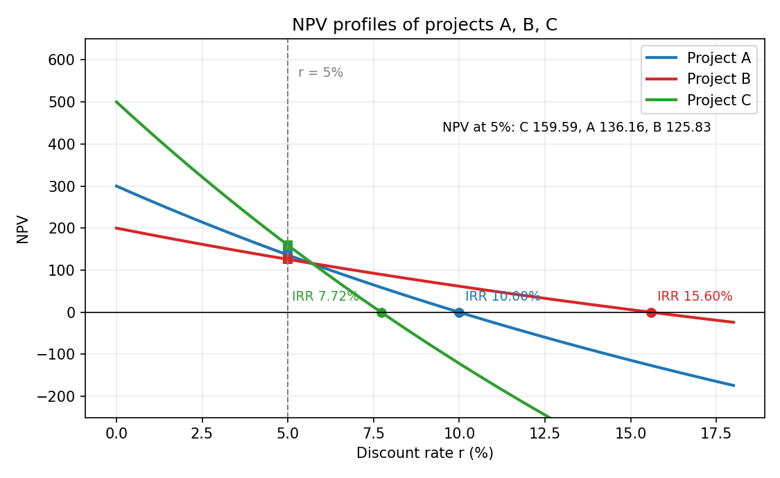
All three have and , so each is worth doing on its own. If only one can be chosen (mutually exclusive), use NPV: it measures the value added in money terms, so choose C.
Intuition: why the two criteria disagreeIRR is a rate of return, blind to scale: B earns a high rate on a small 700 outlay, C a lower rate on a large 2,000 outlay but for all 3 years. NPV counts the value created in money terms, and C creates the most. The profiles also cross: C has the steepest line because its cash comes last, so it wins at low discount rates and loses at high ones. (My own check: the crossover rates are about 5.65% for A against B, 5.71% for C against B and 5.74% for C against A, all just above 5%, so C's lead at 5% is narrow.)
If capital were rationedProfitability Index (NPV per unit invested) would favour B: against for A and for C. This is only relevant if the question mentions a budget limit; the sheet does not.
Q3 — Loan with fees: effective annual rate (sheet 2)
Reconstructed question: the question paper is not on disk. This wording was inferred from the worked spreadsheet; check it against the real paper.
A bank lends 50,000 for 10 months at a stated (nominal) annual rate of 12%, i.e. 1% per month. Interest is paid at the end of each month and the principal is repaid at the end of month 10. The bank charges a fee of 1,000 at the start, deducted from the amount you receive, and a further 1,200 at the end, paid with the final repayment.
a. What are the borrower's cash flows? b. What is the effective monthly rate, and what is the effective annual rate (EAR)?
Input missing from sourceThe workbook enters the 1,200 final fee with no label, so what it represents (closing fee, early-repayment fee) is unknown. I treated it as a fee paid at month 10, as the cell sits there.
AI-written answer, not official. Check before relying on it.
a. Cash flows (borrower's view, months 0 to 10)
| Month | Flow |
|---|---|
| 0 | |
| 1 to 9 | each (interest ) |
| 10 |
b. Effective rates
The monthly cost solves
In Excel: =IRR(B8:L8) gives per month. Check: at this the present value of the payments equals 49,000 (error below ).
Convert to an annual effective rate (Lesson_03-Rate Conversion, Effective Rates & EAC):
Intuition: why 18.73% and not 12%Without fees the loan costs 1% a month, an EAR of (already above the stated 12% because of monthly compounding). The fees mean you receive only 49,000 but still owe 50,000 plus 1,200, which pushes the monthly cost from 1% to 1.44%. Do not multiply 1.44% by 12 (that gives 17.29%): rates compound.
Workbook leftoversCell
B10holdsr_guess = 0.1846, which no formula uses (a leftover starting guess for solving by hand). The workbook's 18.73% matches my result.
Q4 — Equal-payment loan and amortisation table (sheet Sheet4)
Reconstructed question: the question paper is not on disk. This wording was inferred from the worked spreadsheet; check it against the real paper.
A loan of 15,000 is taken at an annual interest rate of 10% and repaid in 5 equal annual payments.
a. Find the annual payment. b. Build the amortisation table (interest, principal repaid and ending balance each year).
AI-written answer, not official. Check before relying on it.
a. The payment
For an equal-payment loan (Lesson_05-The Four Loan Types):
In Excel: =PMT(10%, 5, -15000). (The workbook writes PMT(B2,B3,B1) with the loan positive, so Excel returns and the table flips the sign.)
b. Amortisation table
Each year: interest opening balance, principal interest, ending balance opening principal.
| Year | Opening balance | Interest | Principal repaid | Payment | Ending balance |
|---|---|---|---|---|---|
| 1 | 15,000.00 | 1,500.00 | 2,456.96 | 3,956.96 | 12,543.04 |
| 2 | 12,543.04 | 1,254.30 | 2,702.66 | 3,956.96 | 9,840.38 |
| 3 | 9,840.38 | 984.04 | 2,972.92 | 3,956.96 | 6,867.46 |
| 4 | 6,867.46 | 686.75 | 3,270.22 | 3,956.96 | 3,597.24 |
| 5 | 3,597.24 | 359.72 | 3,597.24 | 3,956.96 | 0.00 |
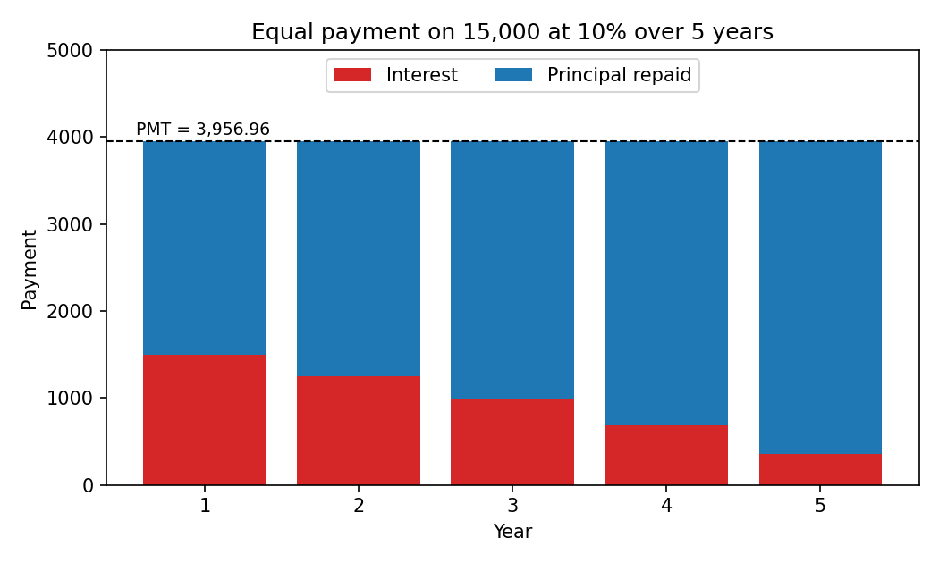
Checks.
- The final balance is 0 (to rounding), so the payment is right.
- The balance after year 3 equals the present value of the two remaining payments: . ✓
- Total interest paid , which equals the sum of the interest column.
- Excel per-year split:
IPMT(10%, t, 5, -15000)andPPMT(10%, t, 5, -15000).
IntuitionThe payment is level, but early on most of it is interest (1,500 of 3,957 in year 1) because the balance is high. As the balance falls the interest share shrinks and the principal share grows.
Q5 — Growing outflows against periodic inflows: NPV (sheet 7)
Reconstructed question: the question paper is not on disk. This wording was inferred from the worked spreadsheet; check it against the real paper.
A project receives an inflow of 20,000 every 3 years, at the ends of years 2, 5, 8 and 11. It has an outflow of 6,000 at the end of year 1, growing at 3% a year, paid at the end of every year from year 1 to year 11 (so 6,180 in year 2, and so on). The discount rate is . Find the NPV.
AI-written answer, not official. Check before relying on it.
Method 1: net cash flow each year, then NPV
Outflow in year is (6,000; 6,180; 6,365.40; ...; 8,063.50 in year 11). Net each year, then discount:
| Year | 1 | 2 | 3 | 4 | 5 | 6 | 7 | 8 | 9 | 10 | 11 |
|---|---|---|---|---|---|---|---|---|---|---|---|
| Inflow | 20,000 | 20,000 | 20,000 | 20,000 | |||||||
| Outflow | 6,000 | 6,180 | 6,365.40 | 6,556.36 | 6,753.05 | 6,955.64 | 7,164.31 | 7,379.24 | 7,600.62 | 7,828.64 | 8,063.50 |
| Net | 13,820 | 13,246.95 | 12,620.76 | 11,936.50 |
In Excel: =NPV(10%, C8:M8). Here the function is used correctly: the first value in the range is year 1 and the flow is zero.
Method 2: closed forms (cross-check)
Outflows, a Growing Annuity with first payment 6,000 at , , 11 payments:
Inflows, four payments discounted one by one:
| Year | 2 | 5 | 8 | 11 |
|---|---|---|---|---|
| 16,528.93 | 12,418.43 | 9,330.15 | 7,009.88 |
(Equivalently, treat the 3-yearly payments as an annuity at the 3-year rate : , the factor 1.1 shifting the valuation date because the first payment is at year 2, not year 3.)
The workbook shows 1,158.71 with no label; it agrees with both methods. Since , the project is worth doing at 10%.
IntuitionCosts arrive every year and keep growing, so they are an annuity that rises. Revenue arrives in lumps every third year. The lumps are large enough that, discounted, they just beat the stream of costs, leaving a small positive NPV.
Summary
Key takeaways
- FCF ; depreciation is a tax shield, working capital is cash tied up then released. Use symmetric tax on losses.
- Excel's
NPVstarts at : write=CF0 + NPV(r, CF1:CFn). The workbook's Q1 NPV of 2,576.18 forgot this; the correct value is 2,756.51.- A
#N/AfromFORMULATEXTon an empty cell is just a label error and changes nothing.- NPV and IRR can rank projects in opposite order; for mutually exclusive projects trust NPV.
- The all-in cost of a loan with fees is the IRR of the borrower's cash flows, then convert to an annual effective rate with .
- Equal-payment loan: ,
PMT; interest opening balance.- For growing costs use the Growing Annuity formula, or net each year and use
NPV.
Related Notes
- Lesson_06-Capital Budgeting & Free Cash Flow · Lesson_02-Perpetuities, NPV & IRR · Lesson_03-Rate Conversion, Effective Rates & EAC · Lesson_05-The Four Loan Types · Lesson_01-Time Value of Money
- HW_07-Free Cash Flow & Project NPV · HW_02-NPV, IRR & Project Choice · HW_04-Effective Interest Rates · HW_06-Loans & Amortization
- Financial Management