
2025 Moed B — Eco-Labeled Apple Demand, Quadratics, Dummies & Chow Test
- #intro-econometrics
- #past-paper
- #exam-prep
- #log-log-model
- #omitted-variable-bias
- #multicollinearity
- #f-test
- #quadratic-model
- #dummy-variable
- #interaction-term
- #chow-test
2025 Moed B — Eco-Labeled Apple Demand, Quadratics, Dummies & Chow Test
Part of: Intro Econometrics Final Exam 2025, Moed B (4 April 2025) — Introduction to Econometrics, Dr. Aluma Dembo. 100 points, 3 hours, open notes (20 pages), significance level 5% unless stated, round to 3 significant figures. Builds on: Lec_08-Goodness of Fit & Multicollinearity, Lec_10-Dummy Variables, Lec_11-Interaction Terms, Lec_13-Exam Review Related assignments: Assign_01-Interpreting OLS Output & the Birthweight-Smoking Regression, Assign_02-Functional Form & the Money-Supply Log-Log Model, Assign_03-Change of Variables, Regression Through the Origin & the Housing Model, Assign_05-Quadratics, Dummy Variables, Interactions & the Chow Test
No official answer key: every answer here is AI-writtenThis paper came without a key. All 16 questions (every sub-part) are AI-solved, with arithmetic re-checked in Python and grounded in Lec_13-Exam Review and the formula sheet. Treat them as carefully reasoned, not official. Q3 (omitted-variable trick), Q7 (what partial multicollinearity does), Q13 (why the intercept changes) and Q5 (units of
income, back-transforming the log) are the ones where the exam's intended wording could differ from mine.
Exam mechanicsEach answer in the real exam goes in a box with "[1 point] answer" plus "[4 points] show your work", so below each answer is followed by its justification. Some output lines in the scan are blacked out (the t value of in model [A]); the tests below rebuild them.
What this paper tests
One paper, the whole coursePart I (47 pts) is a demand for eco-labeled apples story with five nested regressions ([1] to [5]). It tests, in order:
- Logs and elasticities (Q1), unit changes (Q2).
- Omitted-variable bias used backwards: recover a covariance from a short and a long regression (Q3).
- t-tests (one-sided) and predictions (Q4, Q5).
- Perfect vs partial multicollinearity (Q6, Q7) and an F-test for joint significance (Q8).
Part II (53 pts) is an abstract on dataset (113 observations) walking through t-tests / p-values, R² and the F-test of model significance, a quadratic, a dummy, an interaction, a confidence interval and a Chow test (Q9 to Q16).
Intuition: the "find the number in the R output" skillAlmost every number needed is already printed: coefficient, SE, , degrees of freedom, . The marks are for (a) picking the right row, (b) setting up the right and tail, (c) using the right degrees of freedom and critical value.
Part I — Apple demand [47 pts]
Data: 660 survey participants, but 248 were dropped for missing values, so the regressions use observations. (Check: model [1] has 409 residual df and 3 parameters, .) ln.Q.eco, ln.P.eco, ln.P.reg are log quantity of eco apples, log price of eco apples and log price of regular apples; income is in thousands of USD.
Model [1] output (model.1), :
| Variable | Estimate | Std. Error | t | p |
|---|---|---|---|---|
| (Intercept) | 0.62829 | 0.05065 | 12.405 | <2e-16 |
| ln.P.eco | -0.44737 | 0.20678 | -2.163 | 0.0311 |
| ln.P.reg | 0.34362 | 0.21489 | 1.599 | 0.1106 |
Residual SE 0.7107 on 409 df; , adj. ; on 2 and 409 df, p = 0.09263.
Q1 — Price elasticities in a log-log demand model [6 pts]
AI-written answer, not official. Check before relying on it.
AnswerOwn-price elasticity . Cross-price elasticity .
In a Log-Log Model the slope on a logged regressor is the Elasticity: (see Assign_02-Functional Form & the Money-Supply Log-Log Model).
- Own price of eco apples (): a 1% rise in the eco-apple price lowers the quantity of eco apples demanded by about 0.447%, holding the regular-apple price fixed. Demand is inelastic (). The coefficient is significant at 5% (, ).
- Price of regular apples (): a 1% rise in the regular-apple price raises eco-apple quantity by about 0.344%, holding the eco price fixed. Positive sign means the two are substitutes. It is not significant at 5% (), so we can't rule out zero cross-price effect.
IntuitionNegative own-price elasticity is the law of demand. Positive cross-price elasticity says shoppers switch to eco apples when regular apples get dearer.
Q2 — Changing the units from lbs to kg [5 pts]
AI-written answer, not official. Check before relying on it.
Answerdoes not change (stays ). Only the intercept changes.
With : (fewer kg than lb) and (USD per kg is higher than USD per lb). Take logs:
Substitute into model [1]:
So the slopes are unchanged: rescaling a variable that is already in logs only adds a constant to it, and adding a constant to a regressor or to shifts the intercept but never the slope (see Lec_13-Exam Review, section 3.1, and Assign_03-Change of Variables, Regression Through the Origin & the Housing Model). Elasticities are unit-free by construction.
The new intercept (not asked), so the new intercept is . Standard errors and -statistics of the slopes are also unchanged.
Q3 — Covariance of log prices from the short and the long regression [6 pts]
AI-written answer, not official. Check before relying on it.
Given: , and the short regression (omits ): .
Answer.
Idea: the omitted-variable-bias formula, solved for the covariance. The short-regression slope equals the long-regression slope plus the bias (see Lec_13-Exam Review, section 2.3, and Omitted Variable Bias):
Equivalently, regress the omitted variable on the included one: , with , and .
Solving
IntuitionThe short regression gives credit for the effect of the regular price. Since the two prices move together (positive covariance) and regular price pushes eco quantity up (), the short slope is biased upward (from to ), which matches the data. The hint "assume Gauss-Markov holds for [1]" is what lets us treat the long coefficients as the truth.
The variance of () is not needed; it is a distractor (it would be used to compute the correlation: ).
Q4 — Do men buy more eco apples? One-sided t-test [6 pts]
AI-written answer, not official. Check before relying on it.
Model [2] output (model.2) (relevant rows):
| Variable | Estimate | Std. Error | t | p |
|---|---|---|---|---|
| ln.P.eco | -0.4564739 | 0.2087481 | -2.187 | 0.0293 |
| ln.P.reg | 0.3477799 | 0.2158877 | 1.611 | 0.1080 |
| age | 0.0047472 | 0.0025435 | 1.866 | 0.0627 |
| educ | -0.0136075 | 0.0165932 | -0.820 | 0.4127 |
| income | 0.0004573 | 0.0009902 | 0.462 | 0.6444 |
| hh.total | 0.0433196 | 0.0250127 | 1.732 | 0.0841 |
| male | 0.0666397 | 0.0843135 | 0.790 | 0.4298 |
Residual SE 0.7096 on 404 df (248 deleted); ; on 7 and 404 df, p = 0.1361.
A. Hypotheses and test statistic
Answervs (men buy more). .
The claim "men purchase more" is the alternative, so the test is one-sided (right tail). The column already prints .
B. Degrees of freedom
Answer(from the R output: "404 degrees of freedom").
C. Conclusion
AnswerFail to reject at 5%: (one-sided, 404 df).
With 404 df the table value is essentially the normal one, . There is no evidence that men purchase more eco apples, all else equal. (The one-sided p-value is .)
TrapThe R p-value () is for a two-sided test. For you either halve it or compare with the one-sided critical value , not .
Q5 — Prediction from model [3] [6 pts]
AI-written answer, not official. Check before relying on it.
Model [3] output (model.3):
| Variable | Estimate | Std. Error | t | p |
|---|---|---|---|---|
| (Intercept) | 0.4836486 | 0.2987585 | 1.619 | 0.1063 |
| ln.P.eco | -0.4753100 | 0.2072871 | -2.293 | 0.0224 |
| ln.P.reg | 0.3636965 | 0.2148468 | 1.693 | 0.0913 |
| age | 0.0044611 | 0.0025165 | 1.773 | 0.0770 |
| educ | -0.0134439 | 0.0165842 | -0.811 | 0.4180 |
| income | 0.0005289 | 0.0009856 | 0.537 | 0.5918 |
| hh.total | 0.0395334 | 0.0245383 | 1.611 | 0.1079 |
Residual SE 0.7093 on 405 df; ; on 6 and 405 df.
AnswerPredicted , so the predicted quantity is lbs.
Plug in, , age 40, educ 12, income 50 (income is in thousands of USD, so USD is the number ), hh.total 4: lbs.
Traps flagged by the hint "read the variable descriptions"
- Income units: the variable is in thousands, so use , not (using would give an absurd ).
- The prediction is for , not . The "predicted quantity" needs exponentiating. (Strictly, understates the mean of because of the log retransformation; the exam does not ask for the correction.)
- values (2 and 3) are already logs, so don't log them again.
Q6 — Perfect multicollinearity in model [4] [5 pts]
AI-written answer, not official. Check before relying on it.
Model [4] includes hh.total and the four age-band counts hh.0.4, hh.5.17, hh.18.64, hh.65.plus.
AnswerThe four age-band counts add up exactly to the household size: for every household, so one regressor is an exact linear combination of the others. Fix: drop one of them (for example
hh.total, or one age band, which then becomes the omitted/reference band).
Every household member falls in exactly one age band (0-4, 5-17, 18-64, 65+), so the bands partition the household. This is Perfect Multicollinearity: the regressor matrix has less than full column rank, assumption "no perfect collinearity" fails, cannot be inverted and OLS cannot compute unique coefficients (R would return NA for one of them). This is a cousin of the Dummy Variable Trap, with counts instead of dummies.
Fix options and what they mean
- Drop
hh.total(keep the four age counts): the information is all still there since total = sum of bands; each coefficient is then the effect of adding one more person of that age band.- Drop one age band (e.g.
hh.18.64), keephh.total: each remaining band coefficient is the effect of swapping an adult aged 18-64 for a person of that band, holding household size fixed.
Q7 — Partial multicollinearity [5 pts]
AI-written answer, not official. Check before relying on it.
Model [5] replaces the counts with four overlapping dummies has.0.4, has.5.17, has.18.64, has.65.plus (1 if the household has at least one member in that band). These are not mutually exclusive, so there is no exact collinearity. The scan labels the coefficient "", which I read as (has.18.64); the argument holds for any coefficient.
Correlation matrix (cor(...)):
| age | has.0.4 | has.5.17 | has.18.64 | has.65.plus | |
|---|---|---|---|---|---|
| age | 1.0000 | -0.3535 | -0.1962 | -0.6492 | 0.6505 |
| has.0.4 | -0.3535 | 1.0000 | 0.1360 | 0.1755 | -0.1831 |
| has.5.17 | -0.1962 | 0.1360 | 1.0000 | 0.2329 | -0.2002 |
| has.18.64 | -0.6492 | 0.1755 | 0.2329 | 1.0000 | -0.7843 |
| has.65.plus | 0.6505 | -0.1831 | -0.2002 | -0.7843 | 1.0000 |
Answer(iv) cannot say / none of the above.
Why: the strong correlations (for example between has.18.64 and has.65.plus, and with age) show partial multicollinearity. Per Lec_08-Goodness of Fit & Multicollinearity and Lec_13-Exam Review (section 2.1), partial multicollinearity leaves the assumptions intact (the regressors are not exactly collinear), so:
- (i) wrong: is still unbiased. Bias needs (an omitted variable or similar), not correlated regressors.
- (ii) wrong: OLS is still BLUE (Gauss-Markov holds), i.e. still the efficient linear unbiased estimator. What partial collinearity does is inflate the variance , since is high; that is large variance, not a loss of efficiency relative to alternatives.
- (iii) wrong: the standard error is correctly large, not biased downward. If anything, the SE is high; the formula already accounts for the collinearity.
So none of (i) to (iii) is true: the right statement would be "the variance (and SE) of is large but unbiased and correctly estimated".
Judgement callThe exam writer may regard (ii) as the intended "cannot say" trap. Partial collinearity inflates variance, but "not efficient" is false because OLS remains best linear unbiased. I keep (iv).
Q8 — F-test for the four age dummies in model [5] [8 pts]
AI-written answer, not official. Check before relying on it.
Model [5]: .
A. Hypotheses and
Answer(none of the four dummies matters) vs : at least one . restrictions.
B. Restricted model
Answer(the model without the four dummies).
C. Test statistic
Answer.
Working
D. Conclusion
AnswerFail to reject at 5%: (the table value for is about 2.37; ).
The four dummies are not jointly significant, so the data give no support for keeping them. This is the five-step F-test of Lec_13-Exam Review (section 1.7); see F-test.
Part II — on , , [53 pts]
Variables: outcome; ; ; ; dummy (1 if in category ); .
Model [A] (model.A), :
| Variable | Estimate | Std. Error | t | p |
|---|---|---|---|---|
| (Intercept) | 41.275 | 6.746 | 6.118 | 1.48e-08 |
| W | 5.788 | 1.219 | 4.748 | 6.23e-06 |
| X | -12.251 | 2.887 | (blacked out) | (blacked out) |
Residual SE 36.99 on 110 df; , adj. ; on 2 and 110.
Q9 — Reading a t-table [10 pts]
AI-written answer, not official. Check before relying on it.
A. Number of observations [2 pts]
Answer.
Residual df with parameters (). Cross-check: model [B] has 109 df and 4 parameters, also .
B. Significance test of [3 pts]
Answer. . (two-sided, 110 df): Reject at 5%.
The scan blacked out this row; the other rows show that R's is just estimate/SE, so it is rebuilt here. is significantly related to .
C. Test of [3 pts]
Answer. : Fail to reject at 5%.
Test against a non-zero value: subtract the hypothesised value, not zero. R's printed and only test . Critical value (table: 1.98 at 110 or 1.984 at 100).
D. p-value for [2 pts]
Answer, so the p-value is 1.
The null equals the estimate, so the estimate sits exactly at the centre of the distribution: . (The hint "calculate the -statistic first" gives this away.)
Q10 — Model [B]: significance and R² [5 pts]
AI-written answer, not official. Check before relying on it.
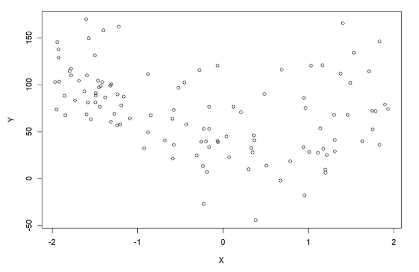
The plot of against from the paper (real data, an image of the source) shows a clear U-shape, which motivates adding .
Model [B] output (model.B), :
| Variable | Estimate | Std. Error | t | p |
|---|---|---|---|---|
| (Intercept) | 8.2912 | 6.8938 | 1.203 | 0.231700 |
| W | 6.9598 | 0.9936 | 7.005 | 2.14e-10 |
| X | -8.4568 | 2.3765 | -3.558 | 0.000554 |
| X.sq | 18.7661 | 2.4130 | 7.777 | 4.48e-12 |
Residual SE 29.8 on 109 df; , adj. ; on 3 and 109 df, p < 2.2e-16.
A. Null hypothesis of the F-statistic [2 pts]
Answer(all slope coefficients are zero; the model has no explanatory power). : at least one slope . The intercept is not included.
B. Percentage of variance explained [3 pts]
Answer, so 52.7% of the variance of is explained by model [B].
Use the multiple , not the adjusted one (adjusted penalises extra regressors and is not "percent of variance explained"). See R-squared and Lec_08-Goodness of Fit & Multicollinearity.
Q11 — The value of X that minimises Y [5 pts]
AI-written answer, not official. Check before relying on it.
Answer.
WorkingHolding fixed, . Second derivative , so this is a minimum (U-shape), and lies inside the observed range .
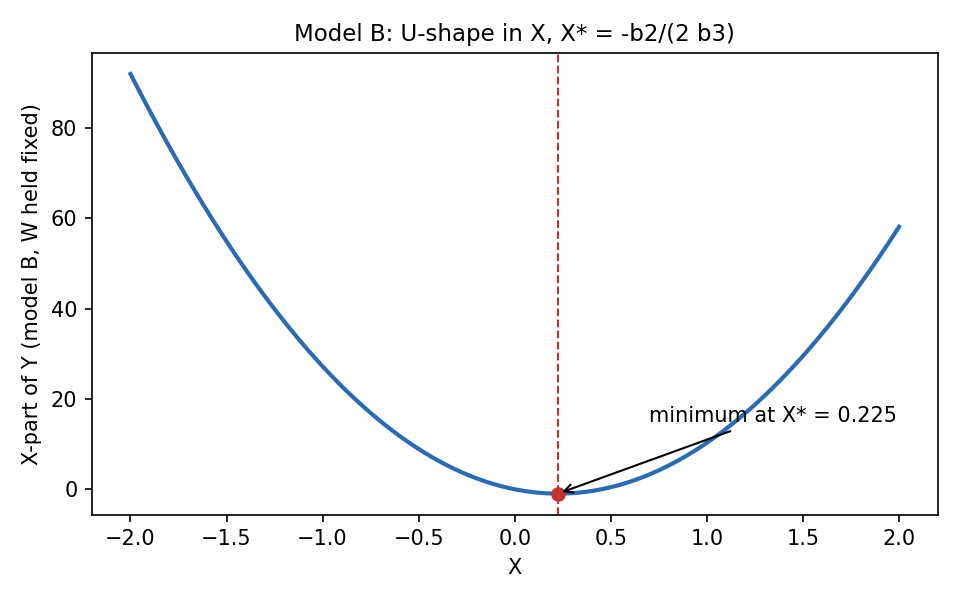
Theory diagram built from the model [B] coefficients: the X-part of the fitted () is a U-shape with its minimum at . See Quadratic Model and Assign_05-Quadratics, Dummy Variables, Interactions & the Chow Test.
IntuitionThe effect of is not constant: it is negative for and positive after, so it does not make sense to talk of "the" marginal effect of (it depends on the level of ).
Q12 — Model [C]: adding the dummy Z [6 pts]
AI-written answer, not official. Check before relying on it.
Model [C] output (model.C), :
| Variable | Estimate | Std. Error | t | p |
|---|---|---|---|---|
| (Intercept) | -14.4700 | 5.4788 | -2.641 | 0.00949 |
| W | 7.5958 | 0.7214 | 10.530 | <2e-16 |
| X | -8.4830 | 1.7187 | -4.936 | 2.92e-06 |
| X.sq | 17.1524 | 1.7525 | 9.787 | <2e-16 |
| Z | 41.1558 | 4.1073 | 10.020 | <2e-16 |
Residual SE 21.55 on 108 df; , adj. ; on 4 and 108.
A. Intercept for observations not in Z [2 pts]
Answer.
With the dummy term vanishes: the intercept is (the base category, see Base Category).
B. Intercept for observations in Z [2 pts]
Answer(26.686).
C. Marginal effect of W [2 pts]
Answerfor both groups.
enters only as an intercept shift, so the two groups share the same slope in : one more unit of raises by about regardless of (parallel lines; see the left panel of the figure under Q14 and Lec_10-Dummy Variables).
Q13 — Why the intercept becomes significant in [C] [5 pts]
AI-written answer, not official. Check before relying on it.
AnswerModel [B] omits , which has a large effect (+41.2 on average) and shifts the level of . The intercept in [B] is not the same parameter as in [C], and the omitted both distorts the estimate and inflates its standard error.
Three things differ between the two intercepts:
- Different meaning. In [C], is the intercept for the non- group (). In [B] it is a blend across both groups, a single common intercept for all observations, pulled up towards the group's level, so its estimate is instead of .
- Omitted-variable bias. strongly affects (, ) and is probably correlated with and , so omitting it biases the included coefficients and the intercept ( shifts from to ; from to ).
- Bigger noise. The omitted goes into the error term, raising the residual SE from (model [C]) to (model [B]) and with it every standard error: the intercept's SE is in [B] versus in [C]. With a small estimate and a large SE, the is in [B] (), but with the corrected estimate and smaller SE it is () in [C].
IntuitionIn [B] the two groups' very different levels are being averaged into one intercept near zero, and the group differences get dumped in the error. Letting each group have its own intercept (with ) removes that noise and reveals that the baseline group sits clearly below zero.
Q14 — Model [D]: interaction between Z and W [6 pts]
AI-written answer, not official. Check before relying on it.
Model [D] output (model.D), :
| Variable | Estimate | Std. Error | t | p |
|---|---|---|---|---|
| (Intercept) | 5.871 | 6.644 | 0.884 | 0.37884 |
| W | 3.622 | 1.077 | 3.362 | 0.00107 |
| X | -9.841 | 1.600 | -6.149 | 1.37e-08 |
| X.sq | 16.614 | 1.609 | 10.327 | <2e-16 |
| Z | 10.638 | 7.540 | 1.411 | 0.16121 |
| W.Z | 6.394 | 1.369 | 4.670 | 8.80e-06 |
Residual SE 19.73 on 107 df; , adj. ; on 5 and 107.
A. Not in category Z [3 pts]
Answer.
B. In category Z [3 pts]
Answer.
Differentiating with respect to gives : set or . The interaction is the extra effect of for the group (, significant), so the slope of in is about three times larger in category . See Interaction Term and Lec_11-Interaction Terms.
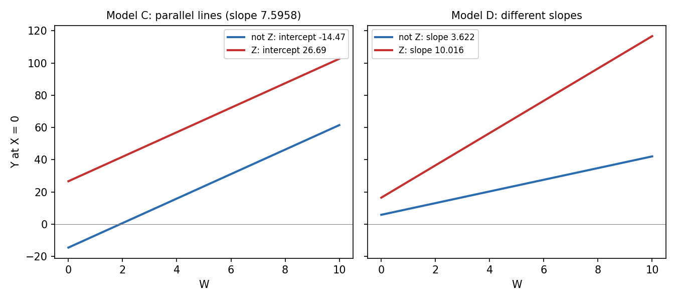
Theory diagram from the printed coefficients (X terms set to 0). Model [C]: only shifts the intercept, so the lines are parallel. Model [D]: the intercepts (5.871 and 5.871+10.638) and the slopes (3.622 and 3.622+6.394) both differ.
Q15 — 90% confidence interval for in model [D] [5 pts]
AI-written answer, not official. Check before relying on it.
AnswerYES, the 90% confidence interval of contains 0. .
Working, , 107 df. For a 90% two-sided interval the critical value is (1.659 exactly; table 1.66 at 100 df). Margin , so the CI is , which contains zero.
Cross-check: the printed , so is not significant at the 10% level, which is equivalent to the 90% CI containing 0. See Confidence Interval.
Q16 — Chow test on model [B] [11 pts]
AI-written answer, not official. Check before relying on it.
Test whether all parameters of model [B] () are the same for and . See Chow Test and Lec_13-Exam Review (section 3.6, version 2: separate regressions).
A. R code for the separate regressions [3 pts]
Answermodel.Z1 <- lm(Y ~ W + X + X.sq, data = sample.data[sample.data$Z == 1, ]) model.Z0 <- lm(Y ~ W + X + X.sq, data = sample.data[sample.data$Z == 0, ])(equivalently
subset(sample.data, Z == 1)orlm(..., data = sample.data, subset = (Z == 1)))
Each regression uses model [B]'s specification, estimated on one group only. The unrestricted model is the pair of regressions; the restricted model is the pooled model [B].
B. F-statistic [6 pts]
Answer.
Working
- (pooled model [B]).
- .
- : the four parameters are restricted to be equal across groups.
- : 113 observations (Q9A) minus 8 parameters (4 for each group).
- .
C. Conclusion [2 pts]
AnswerReject at 5%: (table: about 2.46-2.47).
The regression coefficients differ between category and the rest: the two groups should not be pooled into one quadratic. This is consistent with the significant and terms found above.
Recap table
| Q | Tool | Answer (AI-solved) |
|---|---|---|
| 1 | Log-log elasticities | own (inelastic, significant); cross (substitutes, not significant) |
| 2 | Unit change in logs | unchanged; only the intercept shifts (new ) |
| 3 | OVB formula backwards | |
| 4 | One-sided t-test, 404 df | : fail to reject |
| 5 | Prediction | , lbs (income = 50) |
| 6 | Perfect multicollinearity | counts sum to hh.total; drop one |
| 7 | Partial multicollinearity | (iv): unbiased, still BLUE, variance large but correctly estimated |
| 8 | F-test, | : fail to reject |
| 9 | t-tests | ; reject; fail to reject; p-value 1 |
| 10 | Model F, | ; 52.7% |
| 11 | Quadratic minimum | |
| 12 | Dummy | intercepts and ; slope |
| 13 | OVB / noise | omitted changes the intercept's meaning and inflates its SE |
| 14 | Interaction | effect (not Z), (Z) |
| 15 | 90% CI | : contains 0 |
| 16 | Chow test | R code for two subset fits; , reject |
Related Notes
- Intro Econometrics (hub)
- Lec_08-Goodness of Fit & Multicollinearity, Lec_10-Dummy Variables, Lec_11-Interaction Terms, Lec_13-Exam Review
- Assign_01-Interpreting OLS Output & the Birthweight-Smoking Regression, Assign_02-Functional Form & the Money-Supply Log-Log Model, Assign_03-Change of Variables, Regression Through the Origin & the Housing Model, Assign_05-Quadratics, Dummy Variables, Interactions & the Chow Test