
2025 Moed A — Wage Growth, Dummies, Chow Test & Log Models
- #intro-econometrics
- #past-paper
- #worked-solution
- #dummy-variables
- #interaction-terms
- #chow-test
- #f-test
- #multicollinearity
- #log-models
- #heteroskedasticity
2025 Moed A — Wage Growth, Dummies, Chow Test & Log Models
Part of: Intro Econometrics Final Exam 2025, Moed A (25 Feb 2025, 3 hours, open notes, 100 points) — Introduction to Econometrics, Dr. Aluma Dembo Key concepts: t-test, F-test, p-value, Confidence Interval, Dummy Variable, Base Category, Interaction Term, Quadratic Model, Marginal Effect, Chow Test, Change of Variables, Log-Level Model, Elasticity, R-squared, Adjusted R-squared, Multicollinearity, Heteroskedasticity, White Correction, Regression Through the Origin Builds on: Lec_08-Goodness of Fit & Multicollinearity, Lec_10-Dummy Variables, Lec_11-Interaction Terms, Lec_12-Heteroskedasticity, Lec_13-Exam Review, Assign_03-Change of Variables, Regression Through the Origin & the Housing Model, Assign_05-Quadratics, Dummy Variables, Interactions & the Chow Test
No official key: every answer in this note is AI-writtenThis paper came without a solutions file. All 18 questions (Q1 to Q18) are solved here from the course notes, the formula sheet logic and the R output printed in the paper. Each answer carries its own warning. Check before relying on it. Arithmetic was re-derived in Python. Critical values come from exact
scipyquantiles; the exam expects the printed tables, whose nearest row can differ in the second decimal but never changes a conclusion below.
Format reminderOpen notes. Every multiple-choice answer needs a 1 to 2 sentence justification, so each MC question below gives the verdict, the justification, and why every other option is wrong. Rounding to 3 significant figures is allowed.
What this paper tests
The one idea behind each half
- Part I (52 pts), Thai engineers' wages (N = 403). Everything is about categorical and non-linear regressors: an interaction (
male.educ) gives men and women different education slopes (Q2, Q3); a squared term makes marginal effects depend on the sample point (Q4); the joint F-test is the right test for a whole dummy block (Q7) and for "no growth" (Q5); the Chow test compares separate regressions (Q8); and rescaling units moves coefficients predictably (Q9).- Part II (48 pts),
sample.data(N = 125). The outcome islog(Y), so every coefficient is a log-level one. Themes: a one-sided t-test (Q10), why cannot compare a no-intercept model (Q11, Q12), detecting partial multicollinearity (Q13), confidence intervals (Q14), log-level and elasticity readings (Q15 to Q17), and what heteroskedasticity / White standard errors do to OLS (Q18).- Two traps worth remembering: the base category is the dummy that is missing (Q6), and the of a model with no intercept is not comparable (Q11).
Part I: Wage growth of engineers (52 pts)
Data (N = 403, Thailand, July 1998)
wage(monthly THB),yrs.exp(years at current job),yrs.exp.sq,start.wage,prev.yrs.exp(+ square),educ,is.male,male.educ(=educ×is.male), and degree dummieshs.dropout,hs.grad,polytech,college,post.college.
Q1 — Is prev.yrs.exp.sq irrelevant in Model [1]? (5 pts)
Question. Model [1]:
The R output wage.1 estimates Model [1]. What number lets you conclude prev.yrs.exp.sq does not affect starting wage at ? (1 pt for the number, 4 pts for the explanation.)
R output wage.1 (N = 403, 397 df):
| Term | Estimate | Std. Error | t | Pr(>abs t) |
|---|---|---|---|---|
| (Intercept) | 3393.344 | 2136.125 | 1.589 | 0.1130 |
| is.male | -17752.432 | 2827.402 | -6.279 | 8.96e-10 |
| educ | 669.883 | 168.133 | 3.984 | 8.05e-05 |
| male.educ | 1556.837 | 208.436 | 7.469 | 5.18e-13 |
| prev.yrs.exp | 197.521 | 78.891 | 2.504 | 0.0127 |
| prev.yrs.exp.sq | -2.759 | 2.254 | -1.224 | 0.2217 |
Residual SE 4812 on 397 df; , adj. ; F = 122.6 on 5 and 397 df.
AI-written answer, not official. Check before relying on it.
AnswerThe p-value 0.2217 (equivalently the t-statistic ).
Explanation. Test against . The p-value , so we fail to reject at 1%. Equivalent route: is below the two-sided 1% critical value (about 2.576 from the table's large-df row). So the squared term is statistically indistinguishable from zero.
Intuition"Fail to reject" is not "proved irrelevant". With and SE the data simply cannot tell the coefficient from zero. The question phrases it as "does not affect", which is the conventional reading of failing to reject.
Q2 — Gender-specific models from Model [2] (6 pts)
Question. Model [2]: . Use the output wage.2.
R output wage.2 (398 df):
| Term | Estimate | Std. Error | t | Pr(>abs t) |
|---|---|---|---|---|
| (Intercept) | 3652.6 | 2126.9 | 1.717 | 0.0867 |
| is.male | -17489.3 | 2821.0 | -6.200 | 1.42e-09 |
| educ | 671.2 | 168.2 | 3.989 | 7.88e-05 |
| male.educ | 1553.3 | 208.6 | 7.448 | 5.93e-13 |
| prev.yrs.exp | 105.3 | 23.4 | 4.500 | 8.92e-06 |
Residual SE 4815 on 398 df; , adj. .
AI-written answer, not official. Check before relying on it.
a. Estimated model for men and for women (2 pts)
Answer
- Women (, ):
- Men (, ):
Why. The dummy shifts the intercept by ; the interaction shifts the education slope by . The experience slope is common to both groups.
b. Man, 0 years previous experience, 12 years of education (1 pt)
AnswerTHB
c. Woman, same characteristics (1 pt)
AnswerTHB
d. Man minus woman at 16 years of education, same previous experience (2 pts)
AnswerTHB higher for the man.
CheckMan at 16 years: . Woman at 16 years: . Difference . The previous-experience term cancels, which is why "same previous years of experience" lets you ignore it.
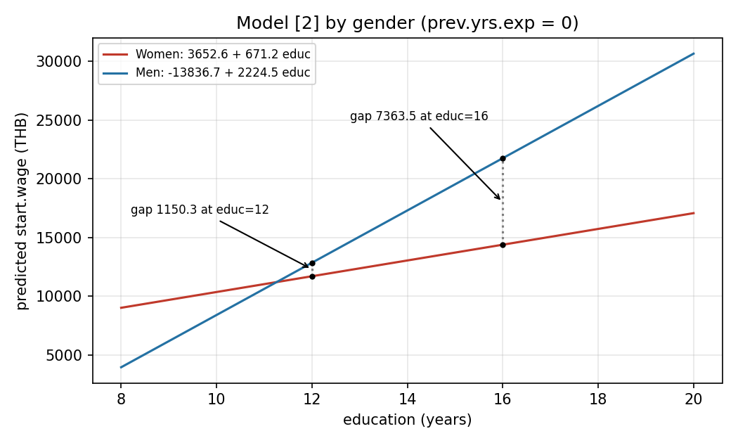
Figure (theory diagram, numbers from the solution): the two fitted lines at prev.yrs.exp = 0. The male line starts far below the female line at low education (negative intercept shift) but is steeper, so the gap opens up from about 12 years of education onward: 1150.3 at 12 years (12857.3 vs 11707.0) and 7363.5 at 16 years.
See Lec_11-Interaction Terms and Assign_05-Quadratics, Dummy Variables, Interactions & the Chow Test.
Q3 — Same marginal effect of education for everyone? (5 pts)
Question. True or false: "In Model [2], the marginal effect of education on starting wage is the same for all observations." (1 pt verdict, 4 pts explanation)
AI-written answer, not official. Check before relying on it.
AnswerFALSE.
Explanation. Because of the interaction :
For women this is THB per extra year; for men it is THB per extra year. It depends on gender (and the interaction is highly significant, ), so it differs across observations. It would be constant only if .
Q4 — Marginal effect of experience in Model [3] (5 pts)
Question. Model [3]: . What is the estimated marginal effect of years of experience on wage? If not constant, evaluate it at the relevant sample average. (1 pt number, 4 pts working)
R output growth.3 (399 df) and means:
| Term | Estimate | Std. Error | t | Pr(>abs t) |
|---|---|---|---|---|
| (Intercept) | 3.974e+04 | 1.791e+04 | 2.219 | 0.02707 |
| start.wage | 1.985e+00 | 5.178e-02 | 38.336 | < 2e-16 |
| yrs.exp | -6.466e+03 | 2.654e+03 | -2.436 | 0.01529 |
| yrs.exp.sq | 2.599e+02 | 9.774e+01 | 2.659 | 0.00814 |
Residual SE 7877 on 399 df; , adj. ; F = 494.3 on 3 and 399 df.
Sample means: wage 34683, yrs.exp 13.51, yrs.exp.sq 185.7, start.wage 17158.
AI-written answer, not official. Check before relying on it.
AnswerTHB per extra year of experience (at the mean ).
Working. yrs.exp appears in two terms, so
depends on the level of experience. Evaluate at the sample mean of yrs.exp (13.51):
Exam trapUse the mean of
yrs.exp(13.51) inside . Do not plug in the mean ofyrs.exp.sq(185.7): the derivative of is , and the mean of the square is not the square of the mean (). Do not use the mean ofwageeither; it is not part of the derivative.
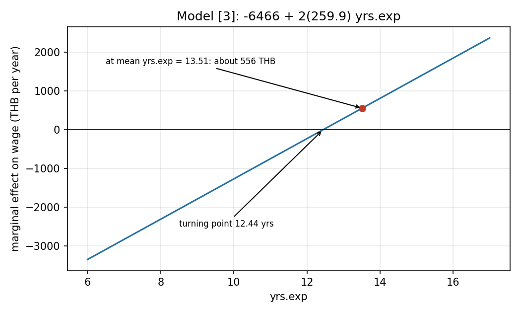
Figure (theory diagram, numbers from the solution): the marginal effect is a straight line in yrs.exp. It is negative below the turning point years and positive above it; at the sample mean of 13.51 years it is about 556 THB.
See Lec_13-Exam Review (quadratic terms) and Assign_05-Quadratics, Dummy Variables, Interactions & the Chow Test.
Q5 — Testing "no wage growth" (5 pts)
Question. Define . How do you test that there is no wage growth in Model [3]? (A) the null in terms of Model [3]'s parameters (3 pts). (B) the restricted model under the null (2 pts).
AI-written answer, not official. Check before relying on it.
a. Null hypothesis (3 pts)
Answer(four restrictions, ). : at least one of these fails.
Why. No growth means exactly (plus noise): on average whatever the experience. Rewrite Model [3] in growth form:
Growth is zero for every value of the regressors only if the intercept, the coefficient on minus one, and both experience coefficients are all zero. Note the restriction on is , not .
b. Restricted model (2 pts)
Answer, equivalently (no parameters at all).
Imposing removes every coefficient (the coefficient is fixed at 1, so it moves to the left side). Because the dependent variable changes from to .
IntuitionEstimate the unrestricted model with as the outcome and test that all coefficients are zero: with and .
See Lec_13-Exam Review (F-test steps: new dependent variable when the null fixes a coefficient at a non-zero value).
Q6 — Model [4]: degree dummies (5 pts)
Question. Model [4]:
R output growth.4 (395 df):
| Term | Estimate | Std. Error | t | Pr(>abs t) |
|---|---|---|---|---|
| (Intercept) | 4.370e+04 | 1.718e+04 | 2.544 | 0.0113 |
| start.wage | 1.581e+00 | 8.777e-02 | 18.014 | < 2e-16 |
| yrs.exp | -6.554e+03 | 2.533e+03 | -2.588 | 0.0100 |
| yrs.exp.sq | 2.604e+02 | 9.327e+01 | 2.792 | 0.0055 |
| hs.grad | 1.130e+03 | 1.450e+03 | 0.779 | 0.4365 |
| polytech | 3.875e+03 | 1.535e+03 | 2.524 | 0.0120 |
| college | 1.025e+04 | 1.915e+03 | 5.355 | 1.46e-07 |
| post.college | 1.122e+04 | 2.422e+03 | 4.634 | 4.88e-06 |
Residual SE 7510 on 395 df; , adj. ; F = 239.2 on 7 and 395 df.
AI-written answer, not official. Check before relying on it.
a. Base category (1 pt)
AnswerHigh-school dropout (
hs.dropout, ).
Why. Five mutually exclusive degree categories, so only four dummies enter. The omitted one is the Base Category, where all four dummies equal 0. Including all five with an intercept would be the dummy-variable trap (perfect multicollinearity).
b. Interpret and (4 pts)
Answer
- (
hs.grad): holdingstart.wageand experience fixed, a high-school graduate earns on average 1,130 THB per month more than a high-school dropout. Not statistically significant (, ): no evidence of a real wage difference between graduates and dropouts at 5% (or 10%).- (
college): holdingstart.wageand experience fixed, a 4-year college graduate earns on average 10,250 THB per month more than a high-school dropout. Highly significant (, below even 0.1%).
Exam trapEach coefficient is a difference relative to the base category (dropouts), not relative to the previous level and not relative to each other. And you must interpret each on its own t-test here; the question explicitly says "not joint".
Q7 — Joint test that highest degree matters in Model [4] (9 pts)
Question. Test that highest degree earned affects wage in Model [4] at . (A) null (1 pt); (B) unrestricted and restricted models (2); (C) degrees of freedom (2); (D) test statistic (2); (E) conclusion with the critical value (2).
AI-written answer, not official. Check before relying on it.
a. Null hypothesis (1 pt)
Answer(highest degree has no effect). : at least one of them is non-zero.
b. Unrestricted and restricted models (2 pts)
Answer
- Unrestricted: Model [4] itself.
- Restricted (this is Model [3]): .
c. Degrees of freedom (2 pts)
AnswerNumerator (four restrictions). Denominator (Model [4] has 8 parameters). So .
d. Test statistic (2 pts)
Both models use the same outcome wage, so the form of the F-statistic works. Restricted is Model [3]'s , unrestricted is Model [4]'s :
Answer(about 11.0).
Cross-check with the residual sums of squaresfor Model [4] (this is the "22280" in Q8, printed in millions). for Model [3] . Then . Same answer; the route is exposed to rounding of the printed (0.788 is only 3 significant figures), so quote about 11.
e. Conclusion (2 pts)
AnswerReject at 1%. Critical value (table: about 3.3 to 3.5 depending on the nearest row). Since , highest degree earned jointly affects wage.
IntuitionJoint significance here is driven mainly by
collegeandpost.college(both highly significant individually), even thoughhs.gradalone is not (Q6b). That is why a dummy block is tested with an F-test, not several t-tests.
See Lec_13-Exam Review (testing a categorical variable jointly) and Lec_08-Goodness of Fit & Multicollinearity (F in form).
Q8 — Chow test: separate models for men and women? (7 pts)
Question. Using the R output below, test whether Model [4] should be estimated separately for men and women. (A) F-statistic (5 pts); (B) conclusion with critical value at 5% (2 pts).
R output (sums of squared residuals, as printed):
| Regression | Sum of squared residuals |
|---|---|
Pooled Model [4] (growth.4) |
22280 |
Men only (is.male == 1) |
17917 |
Women only (is.male < 1) |
3126 |
(The printed values are scaled; the pooled value matches . The units cancel in .)
AI-written answer, not official. Check before relying on it.
a. F-statistic (5 pts)
Chow test, version 2 (separate regressions). Under all coefficients are the same for men and women, so the pooled model is the restricted one:
- : the number of parameters in Model [4] (intercept plus 7 slopes), each allowed to differ by gender
- (two sets of 8 parameters)
Answerwith degrees of freedom.
b. Conclusion (2 pts)
AnswerReject at 5%. (table rows around 120 to infinity: about 1.94 to 2.02). Since , the model differs by gender, so estimate it separately for men and women.
Exam trapThe parameter count is the full parameter count of Model [4] (8, including the intercept), so and the denominator df is . Using 7 (slopes only) or forgetting the doubling are the usual slips.
See Assign_05-Quadratics, Dummy Variables, Interactions & the Chow Test and Lec_11-Interaction Terms.
Q9 — Converting THB to USD (5 pts)
Question. Model [5]: . If both wage and start.wage are converted from THB to USD (1 THB = 0.03 USD), what happens to the estimated marginal effect of education on wage? (1 pt answer, 4 pts working)
R output growth.5 (398 df):
| Term | Estimate | Std. Error | t | Pr(>abs t) |
|---|---|---|---|---|
| (Intercept) | 2.978e+04 | 1.753e+04 | 1.699 | 0.09002 |
| start.wage | 1.742e+00 | 7.035e-02 | 24.763 | < 2e-16 |
| yrs.exp | -6.277e+03 | 2.580e+03 | -2.433 | 0.01541 |
| yrs.exp.sq | 2.519e+02 | 9.501e+01 | 2.651 | 0.00834 |
| educ | 9.518e+02 | 1.927e+02 | 4.939 | 1.16e-06 |
Residual SE 7655 on 398 df; , adj. ; F = 398.5 on 4 and 398 df.
AI-written answer, not official. Check before relying on it.
AnswerIt is multiplied by 0.03: THB per year of education becomes USD per year of education.
Working. Let and the new variables be , . Multiply the whole model by :
So . The coefficients on regressors that are not rescaled (yrs.exp, yrs.exp.sq, educ) and the intercept are multiplied by ; the coefficient on start.wage stays at 1.742 because both and that are scaled by the same (the in the numerator and the from the rescaled cancel).
Standard errors scale with their coefficients, so t-statistics and p-values (and ) do not change.
See Assign_03-Change of Variables, Regression Through the Origin & the Housing Model and Lec_13-Exam Review (unit-change table).
Part II: sample.data (48 pts)
Data (N = 125)and (the R variable is
ln.Y), , , a 0/1 dummy. Note: the printedln.Yvalues run from about to , so the "log" is large in magnitude; the log-level readings in Q15 to Q17 are therefore only approximate (see Q15).
Q10 — Test against 2 in Model [A] (5 pts)
Question. Model [A]: . Test the null that is less than 2 at 10%. (A) test statistic (2 pts); (B) df and critical value (2); (C) conclusion (1).
R output model.A (121 df; the df cell is redacted in the paper but the F line says 3 and 121):
| Term | Estimate | Std. Error | t | Pr(>abs t) |
|---|---|---|---|---|
| (Intercept) | -6.098 | 10.247 | -0.595 | 0.55288 |
| X | -6.733 | 5.610 | -1.200 | 0.23240 |
| W | 4.470 | 4.819 | 0.927 | 0.35552 |
| Z | -12.285 | 4.140 | -2.968 | 0.00362 |
Residual SE 20.74; , adj. ; F = 3.438 on 3 and 121 df, p = 0.01909.
AI-written answer, not official. Check before relying on it.
Which hypothesis?The wording "the null that is less than 2" is read as a one-sided test with the equality in the null: versus . (If you instead set it up as vs , the statistic is the same and the conclusion is also "fail to reject", see below.)
a. Test statistic (2 pts)
Answer.
b. Degrees of freedom and critical value (2 pts)
Answer. One-sided 10% critical value (table row 120: 1.289).
c. Conclusion (1 pt)
AnswerFail to reject at 10%: . No evidence that exceeds 2. (With the opposite orientation, , the rejection region is ; is not in it either: also fail to reject.)
Exam trapThe null is not "", which is the t-value R prints (0.927). You must subtract the hypothesised value 2 first. Use a one-tailed critical value because the hypothesis is one-sided.
See Lec_13-Exam Review (t-test steps, one- vs two-sided).
Q11 — Which comparison shows Model [B] fits better? (5 pts)
Question. Model [B]: (no intercept). Comparing the output for [B] with [A], you conclude [B] fits better. Which comparison supports that?
R output model.B (122 df):
| Term | Estimate | Std. Error | t | Pr(>abs t) |
|---|---|---|---|---|
| X | -8.417 | 4.832 | -1.742 | 0.084048 |
| W | 4.749 | 4.783 | 0.993 | 0.322720 |
| Z | -13.117 | 3.886 | -3.376 | 0.000988 |
Residual SE 20.68 on 122 df; , adj. ; F = 58.42 on 3 and 122 df.
AI-written answer, not official. Check before relying on it.
Answer(v) cannot say / none of the above.
Explanation. Model [B] has no intercept. R computes for a no-intercept model against the uncentred total sum of squares () instead of . Since here is far from zero (mean about ), the uncentred benchmark is huge, which mechanically inflates from 0.079 to 0.590. The two numbers are on different scales, so neither nor adjusted can compare a model with an intercept to one without (Lec_08-Goodness of Fit & Multicollinearity: "models with no intercept").
The only comparable evidence points the other wayCompare residual sums of squares, which are on the same scale: Model [A] versus Model [B] (the
anovain Q13 prints 52181). Model [A] (more flexible, nested) fits at least as well in-sample, and [B]'s tiny residual-SE advantage comes only from using one more degree of freedom.
Each option.
| Option | Verdict | Why |
|---|---|---|
| (i) 0.5896 > 0.07855 | Wrong | Compares an uncentred (no intercept) with a centred . Not comparable. |
| (ii) 0.5795 > 0.05571 | Wrong | Same problem for adjusted : it inherits the uncentred , so the penalty for fewer parameters cannot repair it. |
| (iii) 0.23240 > 0.084048 | Wrong | These are the p-values of in [A] and [B]. A smaller p-value for one coefficient says nothing about overall fit. (And "0.2324 > 0.084" would mean [A] is less significant, not that [B] fits better.) |
| (iv) 4.749 > 4.470 | Wrong | Compares estimates of . Coefficient size is not a goodness-of-fit measure. |
| (v) cannot say / none | Correct | No listed comparison is valid. |
IntuitionDropping the intercept forces the line through the origin. That changes what measures, so its jump is an artefact, the same trap as in Assign_03-Change of Variables, Regression Through the Origin & the Housing Model (Q5c).
Q12 — R code for Model [B] (3 pts)
AI-written answer, not official. Check before relying on it.
Answermodel.B = lm(ln.Y ~ 0 + X + W + Z, data = sample.data)(Equivalent:
lm(ln.Y ~ X + W + Z - 1, data = sample.data).)
Why. Model [B] drops the intercept, and in R's formula syntax 0 + (or - 1) removes it. The outcome variable is called ln.Y in sample.data (as in the model.A call). The output has no (Intercept) row, which confirms it. See Regression Through the Origin.
Q13 — Evidence of partial multicollinearity between and (8 pts)
Question. After seeing Model [B] you suspect and are irrelevant and estimate Model [C]: . Three pieces of evidence together indicate partial multicollinearity between and . (3 pts list; 5 pts how they combine.)
R output (Model [C], F-test and correlations):
| Item | Value |
|---|---|
Model [C] Z coefficient |
-27.202 (SE 2.329, t = -11.68) |
| Model [C] residual SE | 22.1 on 124 df; , adj. |
anova(model.C, model.B) |
Res.Df 124 vs 122; RSS 60540 vs 52181; Df 2; Sum of Sq 8359.1; F = 9.7719; p = 0.0001158 |
| 0.89534 | |
| / | -0.0555 / -0.0654 |
AI-written answer, not official. Check before relying on it.
Answer: the three pieces
- Individually insignificant: in Model [B], neither () nor () is significant at 5%.
- Jointly significant: the F-test of Model [C] against Model [B] () gives , . Reject: and together do matter.
- High correlation: , far above the rule-of-thumb 0.7. ( and are barely correlated with , so the problem is only between those two.)
How they combine (5 pts). The recipe in Lec_13-Exam Review is: neither variable significant on its own, yet jointly significant, and the two are strongly correlated.
- The F-test (evidence 2) says the pair carries real explanatory power, so "X and W are irrelevant" is false. Irrelevance would have shown up as both t-tests and the joint F-test being insignificant.
- Yet the t-tests (evidence 1) say neither one matters when the other is in the model. These two statements are only compatible if the variables share the same information: each is a near-substitute for the other, so the model cannot attribute the effect to either separately.
- Evidence 3 supplies the mechanism: with , the variance inflation factor is . From the standard errors of and are inflated (by about ), pushing their t-statistics toward zero. Estimates stay unbiased; only precision is lost.
- Hence do not drop both (that would throw away real information, as the F-test shows); keep at least one of them.
IntuitionModel [D] (used in Q14 to Q18) keeps only and : becomes highly significant () and adj. stays at 0.5795, exactly as in [B]. That is a fourth, supporting symptom of the same collinearity: once stops competing with it, 's precision returns.
See Lec_08-Goodness of Fit & Multicollinearity and Multicollinearity.
Model [D] for Q14 to Q17Model [D]: (no intercept again).
R output
model.D(123 df):
Term Estimate Std. Error t Pr(>abs t) X -3.6952 0.8577 -4.308 3.33e-05 Z -13.3992 3.8752 -3.458 0.000749 Residual SE 20.68 on 123 df; , adj. ; F = 87.14 on 2 and 123 df.
Sample means: , , , .
Q14 — 95% confidence interval for (5 pts)
AI-written answer, not official. Check before relying on it.
Answer[-5.39, -2.00] (lower , upper ).
Working. with and (table row 120: 1.980):
Lower , upper . Zero lies outside the interval, consistent with being significant at 5% (Lec_13-Exam Review: CI and two-sided test duality).
Q15 — Interpreting (5 pts)
AI-written answer, not official. Check before relying on it.
Answer(ii) A 1 unit increase in decreases by 370%.
Explanation. This is a log-level model: the outcome is , the regressor is in levels. In a log-level model a one-unit increase in changes by approximately percent (Lec_13-Exam Review, log-level row): .
| Option | Verdict | Why |
|---|---|---|
| (i) decreases by 3.70 units | Wrong | That is the level-level reading. is the change in , not in . |
| (ii) decreases by 370% | Correct | Log-level reading: . |
| (iii) a 1% increase in decreases by 370% | Wrong | That is a log-log reading and would need as the regressor. Here is in levels. |
| (iv) decreases by 370% | Wrong | falls by 3.70 log points, not by 370%; the percentage belongs to . |
| (v) cannot say | Wrong | A standard reading exists (ii). |
Caveat on the approximationis a good approximation only for small coefficients. For it breaks down: the exact change is , and a "370% decrease" is impossible for a positive . The alternative (v) is defensible only if the marker insisted on exact percentages. Treat (ii) as the intended answer under the course's approximate rule, and mention the exact figure in your justification if space allows.
Q16 — Interpreting (5 pts)
AI-written answer, not official. Check before relying on it.
Answer(ii) is 1,340% lower for observations in category Z.
Explanation. is a dummy and the outcome is , so is the approximate percentage difference in between category Z and the rest, holding fixed (log-level with a dummy).
| Option | Verdict | Why |
|---|---|---|
| (i) is 13.4 units lower | Wrong | Level-level reading; the effect is on . |
| (ii) is 1,340% lower | Correct | percent, log-level with a dummy. |
| (iii) a 1% increase in decreases by 13.4% | Wrong | is a 0/1 indicator: it cannot rise by 1%. Its coefficient compares two groups. |
| (iv) is 13.4% lower | Wrong | is 13.4 log points lower; the percentage applies to and is , not 13.4%. |
| (v) cannot say | Wrong | A standard reading exists. |
Same caveat as Q15The exact difference is . The approximation is only valid for small , so (ii) is the answer under the course's rule, not a literal 1,340% fall.
Q17 — Elasticity of with respect to (5 pts)
AI-written answer, not official. Check before relying on it.
Answer(a 1% increase in is associated with about a 13.9% fall in ).
Working. In a log-level model the marginal effect is , the rate of change is , and the elasticity is (the log-level row of the moment table in Lec_13-Exam Review). It depends on , so evaluate at the sample mean :
Exam trapThe elasticity is not (that is the log-log answer, wrong here because is not logged). Use the mean of (3.761), not of or .
Q18 — Heteroskedasticity in Model [D] (8 pts)
Question. You suspect heteroskedasticity in Model [D]. All other classical assumptions hold. (A) What does this mean for the OLS estimates? (1 pt MC + 4 pts explanation). (B) You run coeftest(model.D, vcov = hccm, type = "hc0"). (3 pts MC)
AI-written answer, not official. Check before relying on it.
a. Effect on OLS (5 pts)
Answer(iii) The OLS estimator of is unbiased and not efficient.
Explanation. Heteroskedasticity violates A4 (constant error variance) but not A1 or A2 (mean-zero, exogenous errors). Unbiasedness needs only A1 and A2, so stays unbiased. Gauss–Markov efficiency needs A1 to A4, so OLS is no longer BLUE (not efficient): a weighted estimator has smaller variance. In addition the usual standard errors are wrong, so t- and F-tests are invalid (Lec_12-Heteroskedasticity).
| Option | Verdict | Why |
|---|---|---|
| (i) biased and not efficient | Wrong | Bias needs A2 to fail (for example an omitted variable), not A4. |
| (ii) biased and not efficient | Wrong | Same: not biased. |
| (iii) unbiased and not efficient | Correct | A4 fails, so efficiency is lost, but unbiasedness survives. |
| (iv) unbiased and efficient | Wrong | Unbiased, but efficiency is lost (the efficiency claim fails). |
| (v) cannot say | Wrong | The consequence is well defined. |
b. After White standard errors (3 pts)
Answer(iii) The resulting OLS estimator of is unbiased but not efficient.
Explanation. coeftest(..., vcov = hccm, type = "hc0") only recomputes the standard errors (White / heteroskedasticity-consistent). The coefficient estimates are the identical OLS ones, so they remain unbiased and still not efficient; White fixes inference (the SEs, t and p-values), not efficiency. Only weighted least squares, which needs the form of the variance, can restore efficiency (Lec_12-Heteroskedasticity).
| Option | Verdict | Why |
|---|---|---|
| (i) biased and not efficient | Wrong | The point estimates are unchanged and still unbiased. |
| (ii) biased and not efficient | Wrong | Same. |
| (iii) unbiased but not efficient | Correct | OLS point estimates are untouched; only the SEs change. |
| (iv) unbiased and efficient | Wrong | White does not make OLS efficient. |
| (v) cannot say | Wrong | The answer is determined. |
Option (iv) is a trap in both partsOption (iv) in (A) and (B) says is "unbiased and efficient". Half of it is true (unbiased); the exam tests whether you notice that efficiency is the casualty in both cases.
Recap table
| Q | Pts | Tool | Answer (AI-solved) |
|---|---|---|---|
| 1 | 5 | t-test on | p = 0.2217 > 0.01, fail to reject |
| 2 | 6 | Interaction model | Women: 3652.6 + 671.2 educ + 105.3 prev; men: -13836.7 + 2224.5 educ + 105.3 prev; 12857.3; 11707.0; 7363.5 |
| 3 | 5 | Marginal effect with interaction | False: (671.2 women, 2224.5 men) |
| 4 | 5 | Quadratic marginal effect | THB per year |
| 5 | 5 | F-test restrictions | : , , ; restricted: |
| 6 | 5 | Dummies | Base = hs.dropout; (not sig.), (sig.) |
| 7 | 9 | Joint F-test | on (4, 395) > 3.37: reject |
| 8 | 7 | Chow test | on (8, 387) > 1.96: reject |
| 9 | 5 | Change of units | becomes |
| 10 | 5 | One-sided t-test | , df 121, crit 1.289: fail to reject |
| 11 | 5 | comparability | (v): no-intercept not comparable |
| 12 | 3 | R code | lm(ln.Y ~ 0 + X + W + Z, data = sample.data) |
| 13 | 8 | Multicollinearity | Insignificant t's + joint F = 9.77 + cor = 0.895 |
| 14 | 5 | Confidence interval | [-5.39, -2.00] |
| 15 | 5 | Log-level interpretation | (ii) about -370% (approximation) |
| 16 | 5 | Log-level dummy | (ii) about -1340% (approximation) |
| 17 | 5 | Elasticity | |
| 18 | 8 | Heteroskedasticity | (iii) in A and B: unbiased, not efficient |
Related Notes
- Lectures: Lec_08-Goodness of Fit & Multicollinearity, Lec_10-Dummy Variables, Lec_11-Interaction Terms, Lec_12-Heteroskedasticity, Lec_13-Exam Review
- Assignments: Assign_03-Change of Variables, Regression Through the Origin & the Housing Model, Assign_05-Quadratics, Dummy Variables, Interactions & the Chow Test
- Hub: Intro Econometrics