
2023 Moed A — Flight Prices & Omitted Variables
Dataset: Part A: 101,336 TLV departures, June 2021 (price, duration, stops, weekday). Part B: N=78 anonymised sample, Y on X1 and X2
- #intro-econometrics
- #past-paper
- #exam-prep
- #log-log-model
- #t-test
- #f-test
- #dummy-variables
- #interaction-terms
- #chow-test
- #multicollinearity
- #omitted-variable-bias
- #quadratic-model
- #heteroskedasticity
2023 Moed A — Flight Prices & Omitted Variables
Part of: Intro Econometrics Final Exam 2023 — Moed A — Introduction to Econometrics, Dr. Aluma Dembo (15 Feb 2023, 3 hours, open notes, 100 points) Key concepts: Log-Log Model, Elasticity, t-test, p-value, F-test, Dummy Variable, Base Category, Interaction Term, Chow Test, Change of Variables, R-squared, Adjusted R-squared, Multicollinearity, Omitted Variable Bias, Classical Assumptions, Quadratic Model, Marginal Effect, Heteroskedasticity, Residuals Builds on: Lec_08-Goodness of Fit & Multicollinearity, Lec_10-Dummy Variables, Lec_11-Interaction Terms, Lec_12-Heteroskedasticity, Lec_13-Exam Review (covers the whole course, including Lectures 1 to 7 and 9, which have no notes), Assign_02-Functional Form & the Money-Supply Log-Log Model, Assign_03-Change of Variables, Regression Through the Origin & the Housing Model, Assign_05-Quadratics, Dummy Variables, Interactions & the Chow Test
Fully officialThe source PDF contains the paper and the official answer key for all 18 items. Every answer below follows the key. Where the key looks inconsistent with the question wording, the answer is kept and a
> [!warning]shows the check (see Q4, Q5, Q6, Q16, Q17). No question is AI-solved. The one place where I finished a conclusion the key left open is Q16 (flagged there).
Exam rules that shape every answer
- Multiple-choice answers need a 1 to 2 sentence justification or they score 0, so each MC item below gives the verdict, the reason, and why each wrong option is wrong.
- Significance level is 5% unless stated. Numbers may be rounded to 3 significant figures. Use the printed tables, not R's
qt()orqf()(see Lec_13-Exam Review).- Course assumption labels used by the key: A1 mean-zero error, A2 exogeneity , A3 no autocorrelation, A4 homoskedasticity.
What this paper tests
Two datasets, one toolkitPart A (Q1 to Q8), flight prices in logs:
- Q1 to Q3: reading a log-log model (constant elasticity) and the t-test, including testing by rebuilding the t-statistic from the reported SE.
- Q4 to Q6: dummy variables and a base category, a joint F-test written with , and what a change of units does to the coefficients.
- Q7 to Q8: interactions as a test for "different slopes", and a Chow test from separate regressions.
Part B (Q9 to Q18), a small anonymised sample (): 4. Q9 to Q12: an insignificant variable, multicollinearity, omitted variable bias and the bias formula. 5. Q13 to Q16: adding a quadratic, nested F-test with
anova(), marginal effects, one-sided t-test. 6. Q17 to Q18: residual plots, heteroskedasticity/misspecification, and what OLS guarantees about residuals.
The unlocking idea for Part BCompare the three fits.
ols1(Y on X1, X2) has a curved residual plot,ols3(adds ) has a shapeless one and adjusted jumps from 0.215 to 0.810. The true relationship is quadratic in X1, so everything inols1andols2suffers from an omitted variable.
Part A — Flights from TLV (101,336 observations)
Data: Price (NIS) and Duration (minutes) for every departing flight in June 2021.
Q1 — Which model has constant elasticity? [5 pts]
QuestionThe researcher believes the price elasticity with respect to duration is constant. Which model does he use? [2 pts] select one, [3 pts] explain.
Option Model A B C D E F G None of the above / more than one correct
Answer: CIt is a log-log model with price as the outcome, so is the constant elasticity of price with respect to duration.
Why C. In a log-log model , which is the elasticity ( per ) and does not depend on the level of either variable (see Lec_13-Exam Review, section 3.3, and Assign_02-Functional Form & the Money-Supply Log-Log Model).
Why the others are wrong.
- A (level-level): is NIS per minute, so the elasticity changes along the line.
- B (log-level): is a percent change in price per extra minute, not per percent of duration; the elasticity is , which grows with duration.
- D, E, F: price is on the right-hand side (duration is the outcome). F is log-log but it measures the elasticity of duration with respect to price, the opposite direction.
- G: only one option fits, so G is wrong.
Q2 — p-values from t-statistics [6 pts]
QuestionThe estimated slope is 0.958 (t = 249.17) and the intercept is 0.6 (t = 22.97). What can you say about the p-values of the significance tests for and ? [2 pts] select one, [4 pts] explain.
Option Statement A Both p-values are less than 0.01 B p-value below 0.01, p-value above 0.01 C p-value above 0.01, p-value below 0.01 D Both above 0.01 E Cannot say with the information provided
Answer: AIf exceeds the critical value at level , then the p-value is below . With the 1% two-sided critical value is 2.576. Both and are far above it, so both p-values are below 0.01.
Why A. The p-value is the probability of a at least this large under . With about 101,000 observations the t distribution is the standard normal for practical purposes (critical value 2.576 at 1%). A t-statistic of 22.97 is already roughly 9 times the cutoff.
Why the others are wrong. B, C and D each claim that at least one p-value exceeds 0.01, which would need ; neither statistic is close. E is wrong because the table value is all that is needed: a t-statistic plus the degrees of freedom pins down which side of any significance level the p-value falls.
Q3 — Testing [6 pts]
QuestionFrom earlier studies the researcher believes the slope is 1. At which level(s) of significance can be rejected? Use the estimates from Q2. [2 pts] select all correct: , , , not enough information. [4 pts] show your work.
Answer: rejected at 1%, 5% and 10%The reported tests , so first recover the standard error, then build the new t-statistic against 1.
Workingexceeds 2.576 (1%), 1.96 (5%) and 1.645 (10%), so reject at all three levels.
Why "not enough information" is wrong. The standard error is not printed, but it is recoverable from and its t-statistic. Common trap: reusing 249.17 as the statistic for ; that number is only for .
IntuitionStatistical significance is not economic significance: 0.958 and 1 are close, but with 100,000 flights the SE is tiny (0.004), so even a 0.04 gap is "ten standard errors" away.
Model (1) used in Q4 to Q6
Variables: Day (date in June), Stop1, Stop2, Stop3 (dummies, base category = non-stop), day_of_week2 to day_of_week7 (dummies, base category = Sunday).
R output (transcribed):
| Variable | Estimate | Std. Error | t value | Pr(>abs t) |
|---|---|---|---|---|
| (Intercept) | 0.698029 | 0.029452 | 23.70 | below 2e-16 |
| lg.duration | 1.025149 | 0.004984 | 205.67 | below 2e-16 |
| day | -0.000160 | 0.000247 | -0.65 | 0.517 |
| stop1 | -0.601653 | 0.012850 | -46.82 | below 2e-16 |
| stop2 | -0.488720 | 0.014081 | -34.71 | below 2e-16 |
| stop3 | -0.544587 | 0.017891 | -30.44 | below 2e-16 |
| day_of_week2 | -0.020264 | 0.008166 | -2.48 | 0.013 |
| day_of_week3 | -0.031064 | 0.007748 | -4.01 | 6.1e-05 |
| day_of_week4 | -0.005644 | 0.007678 | -0.74 | 0.462 |
| day_of_week5 | 0.002648 | 0.008208 | 0.32 | 0.747 |
| day_of_week6 | 0.003238 | 0.008087 | 0.40 | 0.689 |
| day_of_week7 | -0.068507 | 0.008163 | -8.39 | below 2e-16 |
Residual standard error: 0.674 on 101324 degrees of freedom
Multiple R-squared: 0.398,   Adjusted R-squared: 0.398
F-statistic: 6.09e+03 on 11 and 101324 DF, p-value: < 2e-16
Q4 — Cheapest day of the week [6 pts]
QuestionAccording to model (1), on which day of the week is it cheapest to fly? Consider equal-duration non-stop flights in the same calendar week (e.g. Sunday 6 June to Saturday 12 June 2021). Explain.
Answer: MondayCompare the coefficients: each is the log-price difference relative to the Sunday base. The most negative one, , belongs to Monday in the key's labelling.
Working (as in the key)For a non-stop Sunday flight: .
The same flight on the next day (Monday):
and the day after (Tuesday): , and so on. Since rises by one each calendar day, the term only shifts every weekday by a further per day, which is tiny and insignificant (p = 0.517).
Largest weekday discount: (Monday), then (Wednesday), (Tuesday). Monday is cheapest by a wide margin (roughly 7% below Sunday, from ).
Weekday labelling in the keyThe question says
day_of_week2is Tuesday,day_of_week3is Wednesday and Sunday is the base, which would makeday_of_week7a Sunday again if the numbering simply continued. The key resolves this by readingday_of_week7as Monday. I kept the key's answer (Monday); the dummy numbering in the stem is the sloppy part. The method, picking the most negative dummy coefficient, is what the examiner is testing.
Q5 — Does the number of stops matter? [8 pts]
QuestionThe researcher checks the claim that the number of stops does not affect the price (assuming at least one layover). (A) [2] Null hypothesis? (B) [2] Restricted model? (C) [4] Given of the restricted model , is the claim correct? Show the test statistic and critical value.
a. Null hypothesis
Answer(the coefficients on
Stop1,Stop2,Stop3).
b. Restricted model
AnswerImpose by dropping the three stop dummies:
c. The F-test, written with
Answer: versus critical value , so reject ; the claim is not correctWith restrictions and degrees of freedom the 5% critical value is about 2.6. Since , the stop dummies are jointly significant: the number of stops affects price.
Why the form works. and both models share the same (same dependent variable), so the cancels in the ratio (see Lec_13-Exam Review, section 1.7 and 1.8, and Lec_08-Goodness of Fit & Multicollinearity).
Wording versus the key's hypothesisThe question says "assuming there is at least one layover stop". Read literally, that is a claim that 1, 2 and 3 stops cost the same (, , restricted model = one "any stop" dummy), which would need a different restricted . The key instead tests that all three stop effects are zero relative to non-stop () and supplies for that restricted model. Following the key (the given only fits the "drop all three dummies" model). The coefficients (-0.60, -0.49, -0.54) are all large and negative, so the conclusion is not in doubt either way.
Q6 — Change of units [6 pts]
QuestionHow do the estimates in model (1) change if duration is measured in hours instead of minutes and price in USD instead of NIS? Use an exchange rate of 3.5 USD for every 1 NIS.
Answer (official)The slope on log-Duration, the
Day,Stopand weekday dummy coefficients do not change; only the intercept changes. The key's new intercept is 3.064 (or 1.976 if the exchange rate is applied the other way round; both accepted).
WorkingDuration in hours = Duration in minutes divided by 60. Price in USD is the NIS price scaled by the exchange rate. Because both variables are in logs, a rescaling just adds a constant:
Substituting into model (1), only the constant picks up the extra terms, and the new intercept satisfies
Using the key's numbers (, ):
With the opposite convention for the exchange rate: .
Slopes are unchanged because a log turns a multiplicative rescaling into an additive shift: (see Assign_03-Change of Variables, Regression Through the Origin & the Housing Model and Lec_13-Exam Review, section 3.1).
Which logarithm?The key's constants and are and . If the course's
lg.variables are natural logs, the constants are and and the intercepts would be , that is about 6.15 or 3.64. My check: (key rounds to 3.064). The structure (only the intercept moves) is the same either way. I kept the official numbers.
Q7 — Is the effect of duration different for Europe? [7 pts]
QuestionThe researcher considers flights to Europe and wants to test whether prices there are less affected by duration than prices to other continents. He has
dest_Europe(=1 if the destination is in Europe). (A) [3] Which variable(s) should be added? (B) [4] He adds them and the p-value is below 0.05: what does this say about the coefficient on duration in model (1)? State the hypothesis being tested.
a. Variables to add
AnswerAdd two variables: the dummy
dest_Europeand the interaction .
The dummy shifts the intercept for Europe; the interaction lets the slope on duration differ (see Lec_11-Interaction Terms). A different slope is the hypothesis, but keeping the dummy alongside the interaction preserves the hierarchy of the model and avoids forcing both groups through the same intercept.
b. Reading the result
AnswerThe hypothesis tested is (the duration slope is the same for Europe and elsewhere). A p-value below 0.05 rejects it, so model (1) omits an important variable. That means model (1) has omitted variable bias: the estimate of the duration coefficient (and possibly others) is biased, and it is not efficient.
IntuitionModel (1) forces a single duration slope on every flight. If Europe flights genuinely have a different slope, the single estimate is a blend, correct for neither group.
Q8 — Chow test: Europe versus North America [6 pts]
QuestionModel (1) is estimated separately for the 6,000 flights to Europe and the 6,000 to North America. Pooled RSS ;
anova(fit_EU)residual SS ;anova(fit_N_A)residual SS . Test whether the two destinations share the same pricing model. (A) [2] Degrees of freedom? (B) [2] F-statistic? (C) [2] Conclusion at ?
a. Degrees of freedom
Answer: andThe restricted (pooled) model has 12 parameters; the unrestricted model fits all 12 separately for each group. Hence restrictions (all 12 coefficients equal across groups), and .
b. F-statistic
Answer:Check: numerator , denominator , ratio .
c. Conclusion
Answer: reject, where 2.32 is the closest critical value in the printed table at 1%. Europe and North America do not share the same pricing model.
Version 2 of the Chow testThis uses the separate-regressions form of the Chow test, which the lecture notes prefer when groups may have different error variances: the unrestricted RSS is simply the sum of the two group RSSs (Lec_13-Exam Review, section 3.6; Assign_05-Quadratics, Dummy Variables, Interactions & the Chow Test).
Part B — A colleague's project (, variables Y, X1, X2)
Summary statistics (from summary(sample.data[, c('X1','X2','Y')])):
| X1 | X2 | Y | |
|---|---|---|---|
| Min | 0.8835 | -28.14 | 0 |
| 1st Qu. | 22.4332 | 22.43 | 962 |
| Median | 55.6736 | 52.39 | 1389 |
| Mean | 51.5469 | 49.20 | 1279 |
| 3rd Qu. | 81.0683 | 72.86 | 1645 |
| Max | 99.8656 | 126.95 | 2075 |
Model (1): (ols1)
| Estimate | Std. Error | t value | Pr(>abs t) | |
|---|---|---|---|---|
| (Intercept) | 914.954 | 94.271 | 9.706 | 6.85e-15 |
| X1 | 10.944 | 2.806 | 3.900 | 0.000208 |
| X2 | -4.074 | 2.456 | -1.659 | 0.101303 |
Residual SE 425.3 on 75 df; , adjusted ; F = 11.54 on 2 and 75 DF, p = 4.275e-05.
Model (2): (ols2)
| Estimate | Std. Error | t value | Pr(>abs t) | |
|---|---|---|---|---|
| (Intercept) | 913.309 | 95.347 | 9.579 | 1.05e-14 |
| X1 | 7.088 | 1.590 | 4.457 | 2.82e-05 |
Residual SE 430.2 on 76 df; , adjusted ; F = 19.87 on 1 and 76 DF. cor(X1, X2) .
Q9 — Is X2 significant? [4 pts]
QuestionThe colleague thinks X2 is not significant and should be omitted. [1] Which number(s) did she use? [3] Explain.
AnswerThe p-value for X2: 0.101303 (the t-statistic is also accepted).
It is greater than 0.05, so we cannot reject : the estimate is not statistically significant at the 5% level. If she cites the t-statistic she must compare it with the critical value ( about 1.99 for 75 df, so same conclusion).
Q10 — Why does the fit get worse when X2 is dropped? [6 pts]
QuestionAfter removing X2, goodness-of-fit for model (2) is worse than for model (1). [2] What numbers show this? [4] Normally dropping an insignificant variable improves fit. What might explain the opposite?
AnswerNumbers: adjusted is 0.1968 in
ols2versus 0.2149 inols1.Explanation: X1 and X2 are correlated at 0.828 (above the 0.7 rule of thumb). Including both created partial multicollinearity, which inflates the standard error of X2 and makes it look insignificant. But if X2 truly affects Y, then omitting it from model (2) worsens the fit.
Why the adjusted . Plain can never rise when a variable is dropped (0.2353 to 0.2072). Adjusted penalises the extra regressor, so it is the fair comparison. Here even the penalised measure falls, so X2 is carrying real explanatory power (Lec_08-Goodness of Fit & Multicollinearity).
IntuitionX1 and X2 move together, so the data cannot say how much of the effect is X1 and how much is X2. The pair is jointly useful (overall fit) but individually imprecise (large SE on X2). Insignificance from collinearity is not evidence that the variable is irrelevant.
Q11 — What happens to when X2 is omitted? [5 pts]
QuestionBased on the outputs, what happens to the estimate of when X2 is omitted, and why? Select one.
Option Statement A biased downwards and A1 is violated B biased upwards and A2 is violated C biased downwards and A3 is violated D biased upwards and A4 is violated E None of the above
Answer: EOmitting X2 violates A2 (exogeneity), but the bias is downward: the estimate falls from 10.944 to 7.088. No option pairs "downward" with A2, so none of A to D is right.
Direction of the bias. The bias of the short-regression slope is with (effect of the omitted variable) and (X1 and X2 are positively correlated, 0.828). Negative times positive is negative, so the estimate is biased down, which matches the drop in the estimates (Lec_13-Exam Review, section 2.3).
Why each option fails.
- A: right direction, wrong assumption. A1 (mean-zero errors) is not the one broken; the error now contains and is correlated with X1, which is a failure of A2.
- B: right assumption, wrong direction (upward).
- C: right direction, wrong assumption (A3 is no autocorrelation; the data are an independent random sample).
- D: wrong direction and wrong assumption (A4 is homoskedasticity, not the issue here).
Q12 — Recovering the variance of X1 [4 pts]
QuestionIf , what is the variance of X1?
Answer: (key: 950.5, "around 950 with rounding errors")Use the omitted variable bias formula: short slope = long slope + .
Solve for :
The key writes the coefficients rounded (10.94 and 4.07) and gets the same 950.5; rounding differences move the third digit only.
Q13 — Adding a quadratic term and the nested F-test [6 pts]
QuestionThe colleague suspects a quadratic relationship and uses model (3): . She emails the output below. (A) [2] What null hypothesis does the R code test? (B) [2] Degrees of freedom? (B') [1] Critical value at 5%? (C) [1] Conclusion.
> ols3 = lm(Y ~ X1 + X2 + X1.sq, sample.data)
> anova(ols2, ols3)
Model 1: Y ~ X1
Model 2: Y ~ X1 + X2 + X1.sq
  Res.Df      RSS Df Sum of Sq      F    Pr(>F)
1     76 14063548
2     74  3233078  2  10830470 123.95 < 2.2e-16 ***
summary(ols3):
| Estimate | Std. Error | t value | Pr(>abs t) | |
|---|---|---|---|---|
| (Intercept) | 124.53213 | 69.19819 | 1.800 | 0.076 |
| X1 | 59.72394 | 3.45884 | 17.267 | below 2e-16 |
| X2 | -2.55818 | 1.21108 | -2.112 | 0.038 |
| X1.sq | -0.50026 | 0.03253 | -15.379 | below 2e-16 |
Residual SE 209 on 74 df; , adjusted ; F = 110.7 on 3 and 74 DF.
a. Null hypothesis
Answer: the two variables that
ols3adds tools2(X2 and ) have no effect.
b. Degrees of freedom and critical value
AnswerNumerator ; denominator . Critical value at 5%: 3.15 (3.10 also accepted).
c. Conclusion
Answer: rejectThe test statistic 123.95 is far above 3.15 (equivalently, the p-value is far below 0.05).
Check of the F-statistic from the RSS values
anova(ols2, ols3) is the R version of the nested F-test: the restricted model is the smaller one (Lec_13-Exam Review, section 1.7).
Q14 — Is the marginal effect of X1 always zero? [5 pts]
QuestionThe colleague claims that, based on
ols3, we can reject the null that the marginal effect of X1 on Y is always 0. True, false or cannot say? [1] choose, [4] explain.
Answer: TRUE or CANNOT SAY (both accepted)The marginal effect of X1 is . "Always zero" means and jointly, which needs an F-test that
ols3's output does not report directly. However, both coefficients are individually highly significant (t = 17.267 and -15.379), so the joint test would certainly reject.
Why not a plain t-test. A t-test handles one coefficient. The effect is zero at every X1 only if both pieces vanish, so the hypothesis is joint. When each piece alone is already significant, the joint F-test is also significant (Lec_13-Exam Review, section 1.7).
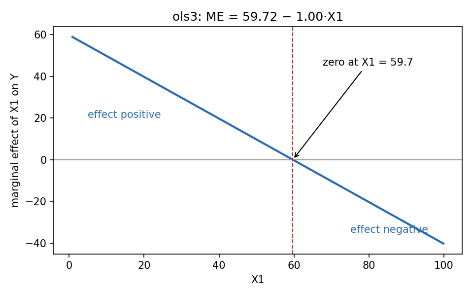
The estimated marginal effect of X1 in ols3 is a straight line that crosses zero at (). It is zero at one point only, but nonzero everywhere else, so "always zero" is rejected.
IntuitionDo not confuse "the effect is zero somewhere" (at the effect changes sign: this is the turning point of the parabola) with "the effect is zero everywhere".
Q15 — Is the rate of return of X2 always negative? [5 pts]
QuestionThe colleague claims that, based on
ols3, the rate of return of X2 on Y is always negative. True, false or cannot say?
Answer: TRUEIn a level-level model the rate of return is the marginal effect divided by the outcome: . The coefficient is negative () and the outcome is positive, so the rate of return is always negative.
Why. Rate of change , which in level-level form is (Lec_13-Exam Review, section 3.3). X2 enters only linearly in ols3, so its marginal effect is the constant and the sign cannot change.
Edge caseThe summary table shows , where the ratio is undefined. The key ignores this and treats Y as strictly positive. I kept the official TRUE.
Q16 — One-sided test on X2 [4 pts]
QuestionTest the null hypothesis that the effect of X2 in model (3) is negative at the level.
Answer (official method)The key's guidance: compare half the p-value to 0.05, or run the full test with the one-tailed 5% critical value. From
ols3: , two-sided , so the one-sided p-value is .
Conclusion not stated in the key (my completion)The key only states the method, not a verdict. With the one-sided method it describes (half the p-value, ), the evidence supports the effect of X2 being negative: we reject in favour of . The critical value for a one-tailed 5% test with 74 df is about , and agrees. Wording caveat: if the null is taken literally as "", the point estimate is already negative and the test would fail to reject; the key's half-p-value instruction only makes sense when the claim to be established is placed in the alternative. I followed the key's method.
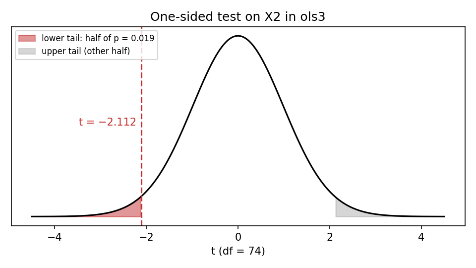
The shaded lower tail beyond holds half of the two-sided p-value (0.019).
Q17 — What can reasonably be said about ols1? [6 pts]
QuestionBased on the residual plots and the outputs of
ols1andols3, which statements are reasonable? [2] select one, [4] explain.
Option Statement A The estimate of in ols1is unbiasedB The standard error of in ols1is biasedC Both A and B are reasonable D Neither A nor B is reasonable
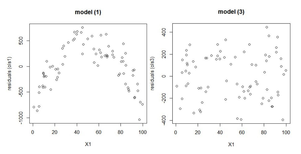
Real data, taken from the exam PDF. Left: ols1 residuals against X1 show a clear arch (curvature) and a wider spread at the ends. Right: ols3 residuals are a shapeless cloud.
Answer: B
ols3fits far better, so it is likely closest to the correct model. Then inols1the estimate of is biased because is omitted, which breaks A2. The plot also suggests heteroskedasticity, which means the standard error of is biased too. Only (B) is reasonable.
Why each option.
- A is wrong:
ols1omits the relevant (the squared term is highly significant inols3), and X1 is correlated with , so the exogeneity assumption fails and the estimate is biased. - B is right: under heteroskedasticity (A4 fails) the usual SE formula is wrong; the key reads the changing spread of residuals in the
ols1plot that way (Lec_12-Heteroskedasticity). - C is wrong because A is wrong. D is wrong because B is reasonable.
Small discrepancy in the keyThe key quotes the adjusted of
ols3as "0.83". The output shows adjusted (), so the figure is slightly off. The argument and the answer (B) do not change.
IntuitionThe arch in the left plot is as much a sign of a missing curvature term (misspecification) as of heteroskedasticity. Either way, the standard errors from
ols1should not be trusted.
Q18 — Residuals in ols1 versus ols3 [5 pts]
QuestionCLAIM 1: the sum of residuals is higher in
ols3than inols1. CLAIM 2: the sum of the squared residuals is lower inols3than inols1. [2] select one, [3] explain.
Option Statement A Only Claim 1 is true B Only Claim 2 is true C Both are true D Neither is true
Answer: BClaim 1 is false: with an intercept, OLS residuals always sum to exactly 0, so the sums are equal in
ols1andols3. Claim 2 is true:ols3has the higher (0.8178 versus 0.2353), and since with the same , its RSS is lower.
Numbers behind Claim 2. From the outputs, and (from anova), which is about 4 times smaller. (Also , consistent with falling when X2 is dropped.)
Why the others are wrong. A and C rely on Claim 1, which is false because the first-order condition for the intercept forces in every OLS model that has a constant. D denies Claim 2, which the comparison confirms.
Recap table
| Q | Topic | Tool | Answer |
|---|---|---|---|
| 1 | Constant elasticity | Log-log | C |
| 2 | p-values from t | t vs 2.576 | A (both below 0.01) |
| 3 | Rebuild t: SE=0.00385 | , reject at 1%, 5%, 10% | |
| 4 | Cheapest weekday | Compare dummy coefs | Monday () |
| 5 | Stops claim | F via , | , reject |
| 6 | Change of units | Logs shift the intercept only | 3.064 (or 1.976) |
| 7 | Europe slope | Dummy plus interaction | Reject, OVB in (1) |
| 8 | Chow EU vs NA | , | , reject |
| 9 | X2 significance | p = 0.101 | Not significant |
| 10 | Fit worsens | Adj , corr 0.828 | Multicollinearity |
| 11 | OVB direction | E (down, A2) | |
| 12 | Variance of X1 | Bias formula | |
| 13 | anova(ols2, ols3) |
Nested F, , | , reject |
| 14 | Marginal effect zero | Joint F | TRUE or CANNOT SAY |
| 15 | Rate of return of X2 | TRUE (negative) | |
| 16 | One-sided X2 | Half p-value | |
| 17 | ols1 reliability |
Residual plot | B |
| 18 | Residuals | Sum is 0; RSS lower | B |
Related notes
- Intro Econometrics (hub)
- Lec_13-Exam Review (whole course), Lec_08-Goodness of Fit & Multicollinearity, Lec_10-Dummy Variables, Lec_11-Interaction Terms, Lec_12-Heteroskedasticity
- Assign_02-Functional Form & the Money-Supply Log-Log Model, Assign_03-Change of Variables, Regression Through the Origin & the Housing Model, Assign_05-Quadratics, Dummy Variables, Interactions & the Chow Test