
2024 Moed B — Experience & Wages, Electricity Cost Function
- #intro-econometrics
- #past-paper
- #exam-prep
- #log-models
- #quadratic
- #dummy-variables
- #omitted-variable-bias
- #r-squared
- #t-test
- #confidence-interval
- #f-test
- #heteroskedasticity
2024 Moed B — Experience & Wages, Electricity Cost Function
Part of: Intro Econometrics Final Exam 2024 — Moed B (18 March, open notes, 3 hours, 100 points) — Introduction to Econometrics, Dr. Aluma Dembo Key concepts: Functional Form, Log-Level Model, Log-Log Model, Quadratic Model, Dummy Variable, Base Category, Omitted Variable Bias, R-squared, t-test, Confidence Interval, p-value, F-test, Heteroskedasticity, Gauss-Markov Theorem Builds on: Lec_08-Goodness of Fit & Multicollinearity, Lec_10-Dummy Variables, Lec_12-Heteroskedasticity, Lec_13-Exam Review, Assign_02-Functional Form & the Money-Supply Log-Log Model, Assign_05-Quadratics, Dummy Variables, Interactions & the Chow Test
No official answer key: every answer here is AI-writtenThere is no key for this sitting. All 15 questions (Q1 to Q15) were solved by AI, grounded in the lecture notes, and every number was recomputed in Python from the R output. Each answer opens with its own warning. Check before relying on any of it, especially the judgement calls flagged in Q1 and Q3.
NumberingThe paper has 15 questions (Part A: Q1 to Q9, 60 points; Part B: Q10 to Q15, 40 points). Page footers read "Page x of 7" and the page-1 instructions are not reproduced below. Each multiple-choice or T/F item needs a 1 to 2 sentence justification in the exam, so every answer below gives one.
What this paper tests
Two datasets, one toolkit
- Part A (wages, n = 27,782): a log-level model with a quadratic, dummies (university is the base) and a control (
iqproxy). Tests: functional form, prediction from output, reading dummies in a log model, unit changes, a t-test against a non-zero value, and omitted-variable bias plus its effect on and the overall F.- Part B (electricity, Cobb-Douglas, df = 94): a log-log model. Tests: reading p-values as "highest significance level", confidence intervals (and their link to tests), elasticities, heteroskedasticity consequences, and a joint F-test written in form.
- Easy marks everywhere: write with the equality, use the right df, and say which assumption fails and which property is lost.
Intuition: the unlocking facts
- In a log-level model, coefficients are approximately percent changes (), and the exact change is .
- Rescaling moves only the intercept in a log model (adds ); slopes are unchanged.
- Dropping a regressor can never raise .
Part A: Experience and wages
Variables: wage (monthly NIS), exp (months of experience), exp_sq, men, iqproxy (psychometric score), private, public, university (the control group).
Q1 — Choosing a functional form [8 pts]
The five-model list on the paper is actually four models:
| Model | |
|---|---|
| i | |
| ii | |
| iii | |
| iv |
A. Linear returns (constant rate of change)
AI-written answer, not official. Check before relying on it.Answer: model (i). Only in model (i) does one extra month of experience add the same NIS amount to the wage at every experience level: , a straight line.
Ambiguous wording"Constant rate of change" could be read in the lecture's sense (, see Lec_13-Exam Review), under which the log-level model (ii) has the constant "rate" . I read "returns are linear" as "the wage-experience relationship is a straight line", which is model (i) only. If the grader accepts (ii) as "constant percentage returns", the answer to A is (i) and (ii), and B is (iii) and (iv).
B. Non-linear returns
AI-written answer, not official. Check before relying on it.Answer: models (ii), (iii) and (iv).
C. Explanation [4 pts]
AI-written answer, not official. Check before relying on it.
- (i) : constant. Linear.
- (ii) : depends on the wage level, so the NIS gain per month changes as wage grows (exponential curve).
- (iii) : depends on both wage and experience. Elasticity is constant, the slope is not.
- (iv) : depends on and can even change sign (turning point).
Model (1) output
lm(formula = ln_wage ~ men + exp + exp_sq + private + public + iqproxy, data = m_data)

             Estimate  Std. Error  t value  Pr(>|t|)
(Intercept)  6.79      0.044       153.81   0.000
men          0.3747    0.0076       48.96   0.000
exp          0.00514   0.002112      2.44   0.015
exp_sq       0.000354  0.000032     11.22   0.000
private      0.1152    0.0094       12.20   0.000
public       0.1063    0.0092       11.48   0.000
iqproxy      0.0022    0.000046     48.51   0.000

Residual standard error: 0.60733 on 27,775 degrees of freedom
Multiple R-squared: 0.3231,  Adjusted R-squared: 0.3230
F-statistic: 2210.02 on 6 and 27775 DF,  p-value: < 0.00000000000000022
and there are 6 slopes, so . See Lec_08-Goodness of Fit & Multicollinearity for reading this output.
Q2 — Predicted wage [6 pts]
Man, exp = 10, iqproxy = 600, private college (so public = 0, university is the base).
AI-written answer, not official. Check before relying on it.Answer: about 5,920 NIS per month ().
| Term | Value |
|---|---|
| intercept | 6.7900 |
| men | 0.3747 |
| exp: | 0.0514 |
| exp_sq: | 0.0354 |
| private | 0.1152 |
| iqproxy: | 1.3200 |
| Sum | 8.6867 |
Note on logsThe model predicts , so you must exponentiate to get a wage. (Retransformation bias, i.e. multiplying by , is not part of this course.) The R output is rounded to 3 sig figs, so expect small differences (roughly 5,900 to 5,950).
Q3 — University man vs public-college woman [6 pts]
AI-written answer, not official. Check before relying on it.Answer: about 30.8% higher (approximation 26.8%).
Same experience and score, so only men, public and private differ:
- University man:
men= 1,private=public= 0, so the group term is . - Public-college woman:
men= 0,public= 1, so the group term is .
Exact versus approximateThe log-level shortcut "" is only accurate for small coefficients. With a gap this large the exact figure is . I give 30.8% as the answer and 26.8% as the quick approximation. If the course expects the shortcut, 26.8% is the likely "official" figure, so show both.
Q4 — Shape of ln(wage) against exp [6 pts]
AI-written answer, not official. Check before relying on it.Answer: (B), an increasing curve that gets steeper (convex).
- The slope is positive at and grows with experience (), so the curve rises and bends upward.
- (A) is a straight line: needs , but is significant ().
- (C) is increasing concave: needs .
- (D) is decreasing concave: needs and .
- (E) is wrong because (B) fits.
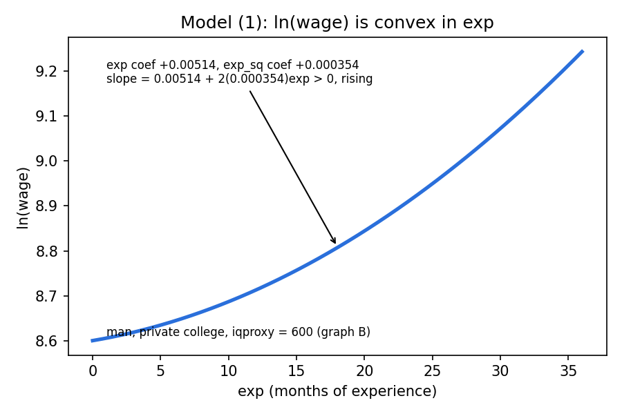
The model (1) fitted curve for a man at a private college with iqproxy = 600, over 0 to 36 months. It is a theory diagram built from the printed coefficients.
IntuitionThe only coefficient pattern that gives (B) is both and positive. A positive squared term means returns to experience are increasing (the minimum of the parabola is at , outside the data).
Q5 — Testing "+100 points raises wage by 20%" [10 pts]
AI-written answer, not official. Check before relying on it.I use the course convention that in a log-level model (change) is the percent change. The exact version is shown at the end.
A. Null hypothesis [3 pts]
A 100-point rise changes by , which is 0.20 for a 20% change:
B. Critical values [2 pts]
Two-sided, (effectively infinite, so use the normal row of the t table):
- :
- :
C. Test statistic [2 pts]
D. Conclusion [1 pt]
, so at we can reject the null.
E. "The p-value is greater than 5%" [2 pts]
FALSE. , so we reject even at 5%, which means (in fact ).
Rounding sensitivityis printed to only 2 significant figures, so the true value could be anywhere in , giving between about 3.3 and 5.4. Every one of those values rejects at 1% and 5%, so the conclusions do not depend on the rounding.
Exact alternativeIf "increase wage by 20%" is read exactly, gives and . Same conclusions (reject at 1%, p-value below 5%).
Q6 — Yearly instead of monthly wage [6 pts]
AI-written answer, not official. Check before relying on it.Answer:
- : increases by (from 6.79 to about 9.275)
- (men): unchanged
- (exp): unchanged
- (exp_sq): unchanged
Yearly wage monthly wage, so
Multiplying the dependent variable by a constant inside a log is just adding a constant to . That shifts the intercept by and leaves every slope alone. This matches the rule in Lec_13-Exam Review: "add constant to : intercept , slope unchanged". Standard errors of the slopes, and the slope t-statistics are all unchanged; only the intercept moves.
IntuitionSlopes in a log-level model are percentages, and a percentage does not care what currency unit or time unit you measure the level in.
Model (2) for Q7 to Q9
Q7 — Effect on the private coefficient [6 pts]
AI-written answer, not official. Check before relying on it.Answer: (B), the estimate of in model (2) is less than in model (1).
Why (omitted-variable bias). Omitting gives
- (estimated 0.0022, ): a higher score raises wages.
- : college graduates (private and public) have lower average scores than university graduates (the base group), so
privateis negatively correlated withiqproxy. - Bias , so the model (2) estimate is below model (1).
Intuition: model (2) credits private with the wage penalty that really belongs to the lower test score, so the private "premium" is understated.
Goodness-of-fit null (asked for in the exam). The overall F-test of model (2): (no regressor explains ), against : at least one is non-zero.
Why not the other options: (A) would need a positive bias (positive correlation); (C) would need or , but both are non-zero; (D) is wrong because (B) holds.
Q8 — R-squared of model (2) versus (1) [6 pts]
AI-written answer, not official. Check before relying on it.Answer: (B), in model (2) is less than in model (1).
with the same (same dependent variable). Dropping a regressor can only keep the same or raise it, so cannot rise. It stays the same only if the dropped variable's coefficient is exactly zero. Here is highly significant (), so the fit worsens strictly.
Null of the goodness-of-fit test: (all slopes zero, restricted model has ).
Why not the others: (A) is impossible (adding variables never lowers , so removing never raises it); (C) needs a zero coefficient; (D) is wrong because (B) holds.
How big is the drop?Dropping one variable is an F-test with . In terms , so . So model (2) has (derived from the printed t, so approximate).
Q9 — Overall F-statistic of model (2) versus (1) [6 pts]
AI-written answer, not official. Check before relying on it.Answer: (B), the F-statistic in model (2) is less than in model (1).
Overall F (from Lec_13-Exam Review):
- Model (1): (matches the printout).
- Model (2): (from Q8), 5 slopes, :
Not a general ruleIn general the overall F can move either way when a variable is dropped: falls (pushes F down) but the numerator df also falls (pushes F up). Here the drop in dominates because is extremely significant, so (B). The comparison relies on derived from , so it is approximate but the gap (about 200) is far larger than rounding error.
Null: for model (2), against : at least one non-zero. Both models reject massively; the question is only how large F is.
Part B: Electricity cost function
= output, = capital price, = wage, = fuel price. Taking logs gives model (1):
              Estimate    Std. Error  t value  Pr(>|t|)
(Intercept)   -8.548757   1.394584    -6.13    0.000
ln_X           0.824102   0.013085    62.98    0.000
ln_pk          0.2028625  [hidden]     [hidden] 0.164
ln_pl          0.1778888  [hidden]     1.25     0.215
ln_pf          0.6932505  0.0807074    8.59     0.000

Residual standard error: 0.21197 on 94 degrees of freedom
Multiple R-squared: 0.9798,  Adjusted R-squared: 0.9790
F-statistic: 1140.68 on 4 and 94 DF,  p-value: < 2.2e-16
Source detailThe standard errors of
ln_pkandln_pland the t-value ofln_pkare hidden by blue boxes on the paper on purpose; they are recovered below from what is shown. With 4 slopes and , observations (the paper mentions 1980 to 2000, which is 21 years, so the data must be several observations per year; this does not affect any answer).
Q10 — Highest significance level at which each variable is significant [6 pts]
AI-written answer, not official. Check before relying on it.Answer: the p-value of each variable.
- : 16.4%
- : 21.5%
- : about 0% (p < 0.001)
A variable is significant at level whenever , so its p-value is the boundary level (see p-value): the smallest at which is rejected. The question's wording is read as asking for this boundary.
Wording caveatStrictly, a variable is significant at every above its p-value, so there is no highest level; the boundary is its p-value. I take that boundary to be the intended answer. For , with 94 df gives , i.e. significant at any conventional level (R prints 0.000).
Q11 — 95% confidence interval for [6 pts]
AI-written answer, not official. Check before relying on it.Answer: about .
The standard error is hidden, so recover it from the printed t-value:
Critical value: two-sided 5%, gives (the printed table row for 90 df gives about 1.99).
(With 1.99 from the table: .) The interval contains 0, which agrees with the insignificant t-test (): the CI and the two-sided test are the same test (Confidence Interval, Lec_13-Exam Review).
Q12 — "0 belongs to the 80% CI for " [6 pts]
AI-written answer, not official. Check before relying on it.Answer: FALSE.
0 lies in the CI exactly when we fail to reject at level . The 80% CI corresponds to . The p-value of is , so we reject at 20%, hence 0 is outside the 80% CI.
Intuition0 would be inside the CI only for confidence levels above . At 80% the interval is narrower than that, so it excludes 0.
Q13 — Doubling output [6 pts]
AI-written answer, not official. Check before relying on it.Answer: cost rises by about 77% (it is multiplied by ). Quick approximation: 82.4%.
In a log-log model is an elasticity: a 1% rise in raises cost by 0.824%. For a doubling (a 100% rise, not small) use the exact form:
Why not 82.4%The " per 1%" reading is a small-change approximation. If the course expects it, the answer would be "about 82.4%", so show both. Also note means economies of scale: doubling output less than doubles cost.
Q14 — Heteroskedasticity (error variance lower before 1990) [7 pts]
Assume the colleague is right, so Assumption A4 (Classical Assumptions, Lec_12-Heteroskedasticity) fails.
| Statement | Answer | Reason |
|---|---|---|
| (A) OLS is unbiased | TRUE | Unbiasedness needs A1 and A2 only (mean-zero error, exogeneity). Changing variance does not touch them. |
| (B) OLS has minimal variance | FALSE | The Gauss-Markov result needs A4. Without it, OLS is not the minimum-variance linear unbiased estimator. |
| (C) OLS is efficient | FALSE | Efficient means smallest variance among unbiased estimators; same reason. |
AI-written answer, not official. Check before relying on it.Justification (4 pts): heteroskedasticity violates A4 only. OLS stays unbiased but loses efficiency (it gives equal weight to noisy and precise observations), and the usual standard errors are biased, so t and F tests are invalid. WLS (variance form known: here, run separate regressions for pre- and post-1990, or weight by the variances) would be efficient; White robust SEs fix the tests but not the efficiency.
(B) versus (C)The paper lists "minimal variance" and "efficient" separately; in this course they both mean "smallest variance among the unbiased estimators", so both are FALSE.
Q15 — Joint test: price of labor and price of capital [9 pts]
AI-written answer, not official. Check before relying on it.
A. Null [1 pt]
B. Restricted model [2 pts]
C. F-statistic [3 pts]
The dependent variable is the same in both models, so the form applies: restrictions, .
D. Critical value and df [2 pts]
(the printed table row for 90 denominator df gives about 3.10). Numerator df = 2, denominator df = 94.
E. Conclusion [1 pt]
, so at we can reject the null: capital and labor prices are jointly significant even though each is individually insignificant (, ). This is exactly the multicollinearity signature (Lec_13-Exam Review, Lec_08-Goodness of Fit & Multicollinearity): high correlation inflates each standard error, hiding the individual effects, but jointly they matter. So the colleague's claim (both affect cost) is supported.
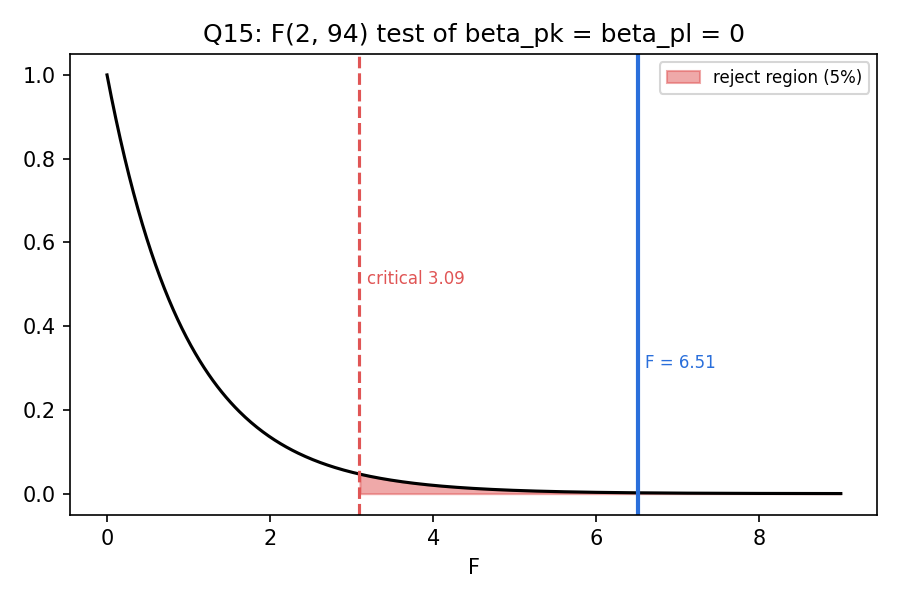
The density with the 5% critical value 3.09 and the computed statistic 6.51 in the rejection region. Theory diagram; the numbers are those of the solution above.
JudgementThe test also supports a more nuanced reading: with -values of 0.16 and 0.22, a high correlation is only a possible cause of the individual insignificance. The F-test shows the two variables matter jointly; it does not by itself prove they are collinear (that would need their correlation).
Recap table
| Q | Topic | Answer (AI-solved) |
|---|---|---|
| 1 | Functional form | A: (i); B: (ii), (iii), (iv) (see ambiguity note) |
| 2 | Prediction | , wage about 5,924 NIS |
| 3 | Dummy gap in a log model | +30.8% exact (26.8% approx) |
| 4 | Shape | (B), convex increasing |
| 5 | t-test | , reject at 1% (crit 2.576); p-value : FALSE |
| 6 | Units | up by ; slopes unchanged |
| 7 | OVB on | (B) smaller |
| 8 | (B) smaller | |
| 9 | Overall F | (B) smaller (about 2,011 vs 2,210) |
| 10 | p-values | 16.4%, 21.5%, about 0 |
| 11 | 95% CI | |
| 12 | 0 in 80% CI of | FALSE () |
| 13 | Double output | cost (+77%); approx +82.4% |
| 14 | Heteroskedasticity | A TRUE, B FALSE, C FALSE |
| 15 | Joint F-test | , reject |