
2023 Moed B — Flight Prices, Chow Test & Multicollinearity
- #econometrics
- #past-paper
- #exam-prep
- #dummy-variables
- #log-log-model
- #interaction-terms
- #chow-test
- #f-test
- #multicollinearity
- #heteroskedasticity
- #quadratic-model
- #units-of-measurement
2023 Moed B — Flight Prices, Chow Test & Multicollinearity
Part of: Intro Econometrics Final Exam 2023 — Moed B — Intro Econometrics, Dr. Aluma Dembo (17 questions, 100 points, open notes, 3 hours) Key concepts: Dummy Variable, Base Category, Log-Log Model, Elasticity, Interaction Term, Confidence Interval, p-value, t-test, F-test, Chow Test, Heteroskedasticity, Weighted Least Squares, Robust Standard Errors, Multicollinearity, Omitted Variable Bias, Quadratic Model, Regression Through the Origin, Residuals, Change of Variables Builds on: Lec_08-Goodness of Fit & Multicollinearity, Lec_10-Dummy Variables, Lec_11-Interaction Terms, Lec_12-Heteroskedasticity, Lec_13-Exam Review; practice in Assign_02-Functional Form & the Money-Supply Log-Log Model, Assign_03-Change of Variables, Regression Through the Origin & the Housing Model, Assign_05-Quadratics, Dummy Variables, Interactions & the Chow Test
No official answer key: every answer in this note is AI-writtenThere is no official solution for this sitting, so all 17 questions (Q1 to Q17) were solved from scratch, grounded in the lecture notes, and every number was recomputed in Python. Treat them as well-reasoned, not official. Check before relying on them. The questions where I am least sure are Q5c (the F-test is very sensitive to R² rounding), Q8 (what "biased" means here), Q9 (which restricted model "pools" the data), Q13 (option B vs C) and Q16 (the premise).
DateThe header says "March 22" with no year; the title says 2023. This note uses 2023 Moed B.
What this paper tests
Two datasets, one toolkit
- Part A (Q1 to Q9) — 3,948 Ben Gurion flights. Reading dummy-variable coefficients (Q1), CIs and t-tests (Q2, Q3), heteroskedasticity and WLS (Q4), an F-test for joint exclusion (Q5), a log-log marginal effect (Q6), interactions (Q7, Q8) and a Chow test (Q9).
- Part B (Q10 to Q17) — an anonymised dataset (n = 120). Multicollinearity (Q10), a merged regressor and an F-test of equal coefficients (Q11, Q12), robust SEs (Q13), residual vs error (Q14), a quadratic peak (Q15), omitting the intercept (Q16) and changing units (Q17).
- Every multiple-choice answer needs a 1 to 2 sentence justification in the real exam. The justifications below are written to that standard.
Reading R output fast
Estimate / Std. Error = t value. Two-sided p-value below 0.05 means "reject H0: coefficient = 0 at 5%". A coefficient on a dummy is a difference from the base category, never a level.
Part A — Flights from Ben Gurion
Variables: Price (NIS), Duration (minutes), Date (1 to 31), EU, AS, AF (destination dummies, base = North America), weekday dummies (base = Sunday). N = 3,948 direct flights.
Q1 — Dummy variables and the model-1 output [6 pts]
Question. Model (1): .
Coefficients:
            Estimate Std. Error t value Pr(>|t|)
(Intercept)   2225.2      32.7    68.0   <2e-16 ***
EU           -1835.9      37.4   -49.0   <2e-16 ***
AF           -1028.4      77.0   -13.3   <2e-16 ***
AS           -1636.9      38.2   -42.9   <2e-16 ***
(A) [3 pts] What is the average price of a direct flight to each of the four destination continents? (B) [3 pts] She wants to test whether the average price to Europe equals the average price to Asia. What null hypothesis should she test?
a.
AI-written answer, not official. Check before relying on it.
With only mutually exclusive dummies and no other regressors, the fitted value for each group is that group's sample mean.
| Destination | Calculation | Average price (NIS) |
|---|---|---|
| North America (base) | intercept | 2225.2 |
| Europe | 2225.2 − 1835.9 | 389.3 |
| Africa | 2225.2 − 1028.4 | 1196.8 |
| Asia | 2225.2 − 1636.9 | 588.3 |
IntuitionThe intercept is the base category's mean. Each dummy coefficient is "this continent's mean minus the base mean". Never read 389.3 as a coefficient; it is the sum.
b.
AI-written answer, not official. Check before relying on it.
Mean price to Europe is and to Asia is . They are equal when
Answer(equivalently ), against . The estimated difference is NIS (Europe is 199 NIS cheaper than Asia on average).
How she would run itThis is a test on one linear combination of coefficients. The output does not give the covariance of , so she either uses an F-test on , or re-estimates with Europe as the base category and reads the t-test on
AS. Not needed for the answer.
Background: Lec_10-Dummy Variables, Dummy Variable, Base Category.
Q2 — 99% vs 95% confidence interval for Monday [5 pts]
Question. Model (2) output (reproduced here, since Q3 to Q6 use it):
log(Price) = b0 + b1 log(Duration) + b2 Date + b3 EU + b4 AS + b5 AF + g1..g6 (Mon..Sat dummies)

              Estimate Std. Error t value Pr(>|t|)
(Intercept)   4.34400    0.17720   24.52   <2e-16 ***
lg.duration   0.49694    0.02613   19.02   <2e-16 ***
date         -0.00144    0.00120   -1.20    0.229
EU           -1.24686    0.04449  -28.02   <2e-16 ***
AF            0.01660    0.07073    0.23    0.814
AS           -0.65252    0.05641  -11.57   <2e-16 ***
Monday       -0.07894    0.03651   -2.16    0.031 *
Tuesday       0.02036    0.03606    0.56    0.572
Wednesday    -0.03635    0.03563   -1.02    0.308
Thursday      0.05510    0.03550    1.55    0.121
Friday       -0.00113    0.03837   -0.03    0.976
Saturday     -0.03988    0.04227   -0.94    0.345

Residual standard error: 0.637 on 3936 df
Multiple R-squared: 0.515, Adjusted R-squared: 0.513
F-statistic: 379 on 11 and 3936 DF
The researcher claims the 99% CI for the coefficient on Monday includes 0 but the 95% CI does not. TRUE or FALSE? Explain.
AI-written answer, not official. Check before relying on it.
Answer: TRUEThe Monday p-value is 0.031. A CI at level excludes 0 exactly when . Here , so 0 is outside the 95% CI but inside the 99% CI.
Check with the numbers (df = 3936, so critical values are essentially normal):
| Level | Interval | Contains 0? | |
|---|---|---|---|
| 95% | 1.961 | (−0.1505, −0.0074) | No |
| 99% | 2.577 | (−0.1730, +0.0151) | Yes |
IntuitionA higher confidence level means a wider interval, so it can only gain values (like 0), never lose them. A coefficient significant at 5% but not at 1% has p between 0.01 and 0.05.
Background: Confidence Interval, p-value, Lec_13-Exam Review (section 1.6).
Q3 — Does price fall as the date moves towards late summer? [6 pts]
Question. She claims the price goes down as the departure date nears late summer (July/August). Test this using the model-(2) output. State the null explicitly.
AI-written answer, not official. Check before relying on it.
The claim is directional ("goes down as Date rises"), so use a one-sided test on the coefficient of Date.
- (price does not fall with the date)
- (price falls with the date: her claim)
- Test statistic: (given).
- One-sided p-value: half the two-sided 0.229, i.e. . Critical value: at 5% one-sided.
Answer(equivalently ), so we fail to reject . There is no statistically significant evidence that price falls with the date. The point estimate is negative (about −0.14% per day) but indistinguishable from 0.
TrapThe data cover June only. Even a significant
Datecoefficient says nothing certain about July and August. Also, the coefficient is in a log-level form, so means about −0.144% per extra day, not −0.00144 NIS.
Background: t-test, Hypothesis Testing, Log-Level Model.
Q4 — WLS and the properties of estimators [3 pts]
Question. She plots price (y) against duration (x) and concludes model (2) has heteroskedasticity. If she corrects with weighted least squares, what happens to the estimators' properties? (A) unbiased, not efficient; (B) biased and not efficient; (C) unbiased and efficient; (D) none of the above. Explain.
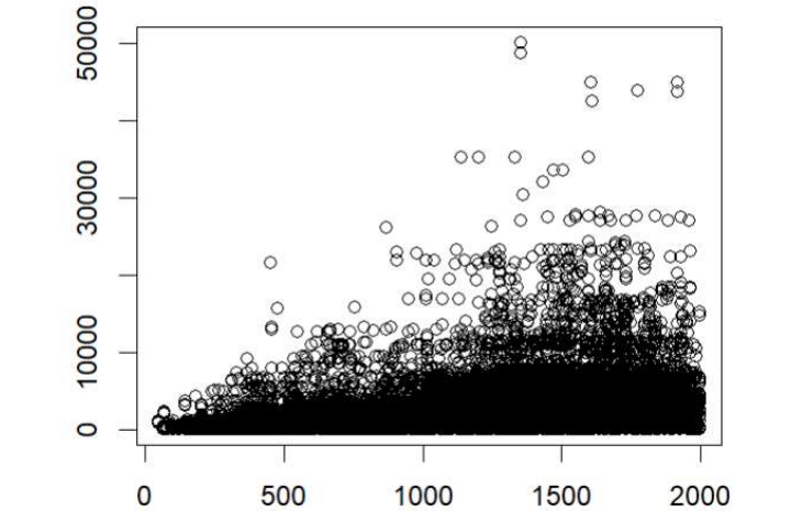
Real data from the exam: the spread of price grows with flight duration (a fan shape), the classic sign of heteroskedasticity.
AI-written answer, not official. Check before relying on it.
Answer: (C) unbiased, and efficientJustification: heteroskedasticity does not bias OLS, and WLS (weights built from the variance pattern, a function of the regressors) keeps unbiasedness while restoring efficiency (it is BLUE when the weights are right).
| Option | Verdict | Why |
|---|---|---|
| (A) unbiased, not efficient | Wrong | This describes OLS under heteroskedasticity (before the fix), not WLS. |
| (B) biased and not efficient | Wrong | Weights depend on the regressors, not the error, so WLS does not introduce bias. |
| (C) unbiased and efficient | Correct | Unbiased, and lowest variance among linear unbiased estimators when the weights match the true variance. |
| (D) none of the above | Wrong | (C) is right. |
CaveatIf the weights have to be estimated (feasible WLS), efficiency holds asymptotically, not exactly. The exam wants (C). Also, the plotted variables are price (not log price) against duration, so strictly it is evidence about the level model; the question tells us to accept the conclusion.
Background: Lec_12-Heteroskedasticity, Heteroskedasticity, Weighted Least Squares, Gauss-Markov Theorem.
Q5 — Joint test: no effect of day of week or date [8 pts]
Question. Test the claim that price is unaffected by either the day of the week or the calendar date. (A) null hypothesis; (B) restricted model; (C) given that the restricted model's , test the claim at any significance level.
a. Null hypothesis [2 pts]
AI-written answer, not official. Check before relying on it.
Answer(the coefficients on
Date, Monday, ..., Saturday). : at least one is non-zero. That is restrictions.
b. Restricted model [2 pts]
AI-written answer, not official. Check before relying on it.
AnswerDrop
Dateand all six weekday dummies:
c. F-test [4 pts]
AI-written answer, not official. Check before relying on it.
Use the form of the F statistic. Unrestricted , restricted , , (from the output).
Critical value .
Answer, so reject at 5%: the day of week and/or the date jointly affect price. (Exam-intended calculation.)
Rounding sensitivity: low confidenceThe two values are rounded to 3 digits, so their difference (0.002) is accurate only to within about ±0.001. The true F ranges from about 1.16 to 3.48 depending on the hidden digits, which straddles the critical value. As a plausibility check, adding the squared t-statistics of the seven excluded variables gives about 10.7, an approximate F of about 1.5, which would fail to reject. The exam says "use whichever significance level you like", so the graded answer is the formula, with the stated conclusion. A careful answer would state the F, the critical value and the caveat.
IntuitionDropping variables always lowers . The F-test asks whether the drop is bigger than chance. Seven variables for a 0.002 drop is a tiny loss, which is why this is borderline.
Background: F-test, R-squared, Lec_13-Exam Review (section 1.7), Lec_08-Goodness of Fit & Multicollinearity.
Q6 — Marginal effect of duration on price [4 pts]
Question. What is the marginal effect of flight duration on the price (at the average value)? Average price 1800 NIS, average duration 1000 minutes.
AI-written answer, not official. Check before relying on it.
In the log-log model is the elasticity: . Rearranging for the effect in NIS per minute:
AnswerAbout 0.894 NIS per extra minute of flight time (at the average flight). Equivalently, a 1% longer flight (10 minutes) is about 0.497% more expensive (about 8.9 NIS).
Background: Elasticity, Marginal Effect, Assign_02-Functional Form & the Money-Supply Log-Log Model.
Q7 — Prediction from the interaction model [5 pts]
Question. Model (3) adds log(Duration) interacted with EU, AF, AS:
              Estimate Std. Error t value Pr(>|t|)
(Intercept)   12.30519    2.37983    5.17 2.4e-07 ***
lg.duration   -0.70915    0.36029   -1.97 0.04911 *
date          -0.00157    0.00119   -1.33 0.18521
EU            -7.72337    2.39532   -3.22 0.00127 **
AF            -5.69134    2.43623   -2.34 0.01953 *
AS            -9.43989    2.38502   -3.96 7.7e-05 ***
Monday        -0.06669    0.03614   -1.85 0.06507 .
Tuesday        0.02601    0.03569    0.73 0.46608
Wednesday     -0.02387    0.03528   -0.68 0.49866
Thursday       0.06300    0.03517    1.79 0.07328 .
Friday         0.00754    0.03798    0.20 0.84267
Saturday      -0.03029    0.04184   -0.72 0.46913
lg.duration:EU 0.92974    0.36372    2.56 0.01062 *
lg.duration:AF 0.79459    0.37237    2.13 0.03291 *
lg.duration:AS 1.37621    0.36168    3.81 0.00014 ***
Residual standard error: 0.63 on 3933 df; R-squared 0.525; Adj. R-squared 0.524
F-statistic: 311 on 14 and 3933 DF
Predict the price of a flight to Europe, 6 hours, departing Sunday 6 June.
AI-written answer, not official. Check before relying on it.
Set: EU = 1, AF = AS = 0, Duration = 6 × 60 = 360 minutes, Date = 6, Sunday is the base, so all weekday dummies = 0.
with :
| Piece | Value |
|---|---|
| Intercept + EU | 12.30519 − 7.72337 = 4.58182 |
| Duration slope for Europe: (−0.70915 + 0.92974) × 5.8861 | 0.22059 × 5.8861 = 1.29841 |
| Date: −0.00157 × 6 | −0.00942 |
| Predicted log price | 5.8708 |
AnswerAbout 355 NIS (log price 5.87).
Retransformationestimates the median price. The mean would be larger by roughly (about 432 NIS with ). The exam expects the simple exponential.
Background: Lec_11-Interaction Terms, Interaction Term, Prediction.
Q8 — Is the model-(2) elasticity biased upwards for Europe? [5 pts]
Question. The researcher claims that in model (2) the estimated elasticity of price w.r.t. duration is biased upwards for flights to Europe. Is the claim correct given model (3)? TRUE or FALSE, explain.
AI-written answer, not official. Check before relying on it.
In model (3) the elasticity depends on the destination:
| Destination | Elasticity from model (3) |
|---|---|
| North America (base) | −0.709 |
| Europe | −0.70915 + 0.92974 = 0.221 |
| Africa | −0.70915 + 0.79459 = 0.085 |
| Asia | −0.70915 + 1.37621 = 0.667 |
Model (2) forces one elasticity for everyone: 0.497. It is a weighted average of the four, dominated by the destinations with many flights.
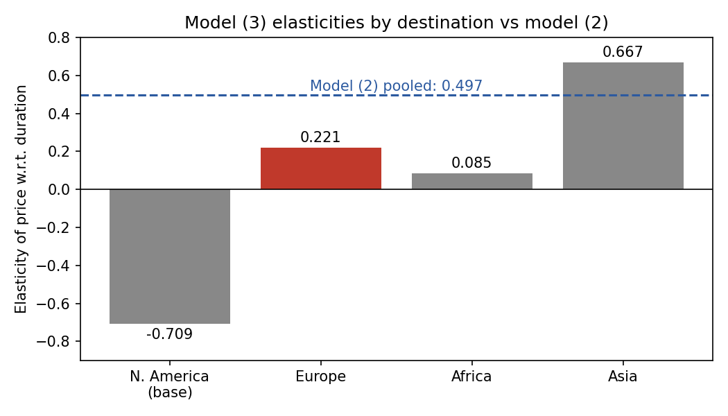
Elasticities implied by model (3) for each continent (derived from the model-3 coefficients), against the single pooled model-2 value 0.497.
Answer: TRUEThe interaction terms are significant (p = 0.011, 0.033, 0.0001), so the common slope in model (2) is misspecified: it omits the interactions, an Omitted Variable Bias problem. Taking model (3) as the better model, the Europe elasticity is 0.221, but model (2) reports 0.497, so for Europe it overstates the elasticity (upward bias of about 0.28).
Caveats
- "Biased" is judged by comparing point estimates: model (3) is itself an estimate (the Europe elasticity has a standard error we cannot compute without the covariance of the two coefficients), so the gap is not formally tested.
- The upward direction is only for Europe: for Asia (0.667) model (2) is too low, and for North America (−0.709) it is much too high. The claim is about Europe, so it is true.
Background: Omitted Variable Bias, Lec_11-Interaction Terms, Assign_05-Quadratics, Dummy Variables, Interactions & the Chow Test.
Q9 — Chow test across continents [8 pts]
Question. Estimate model (2) separately for each continent (EU, AS, AF, NOA; regressors: lg.duration, date, six weekday dummies). Residual sums of squares:
| Continent | RSS |
|---|---|
| EU | 802.6 |
| AS | 666 |
| AF | 5.457 |
| NOA | 69.98 |
| Pooled (all four together) | 1599 |
(A) number of restrictions; (B) ; (C) F critical value at 5%; (D) F statistic; (E) conclusion.
AI-written answer, not official. Check before relying on it.
Setup. Each continent regression has parameters (intercept, lg.duration, date, 6 weekdays). Four groups give unrestricted parameters. : all four continents share the same coefficients (one pooled model).
a. Restrictions [2 pts]
Answerrestrictions (each of the 9 coefficients is equal across the 4 groups: 3 equalities each).
b. Degrees of freedom [1 pt]
Answer.
c. Critical value [2 pts]
Answer(about 1.5; the formula-sheet table for large denominator df gives roughly 1.5).
d. F-statistic [2 pts]
Answer.
e. Conclusion [1 pt]
Answer, so at we can reject the null: the four continents do not share one model; each continent needs its own coefficients.
Ambiguity: which pooled model?The question does not say whether the pooled RSS of 1599 comes from a model with continent dummies. If it does, the intercepts are allowed to differ and only 24 slopes are restricted: , , critical value . The conclusion is the same (reject). I used the textbook Chow test (everything may differ, ). Note that model (2) has RSS , close to 1599, which hints at the continent-dummy version, so be ready for either count.
IntuitionThe Chow test asks whether splitting the data cuts the RSS by more than chance. Splitting cut it from 1599 to 1544, a big enough drop for 27 extra parameters.
Background: Chow Test, Chow-Fisher Test, Lec_11-Interaction Terms, Assign_05-Quadratics, Dummy Variables, Interactions & the Chow Test.
Part B — The colleague's NDA dataset (n = 120)
Outcome , regressors , 120 independent random draws.
Summary statistics (as printed):
| X1 | X2 | X3 | Y | |
|---|---|---|---|---|
| Min | 4.005 | 0.05487 | −14.58 | −1227.7 |
| Mean | 50.017 | 51.84163 | 44.16 | 764.0 |
| Max | 99.866 | 97.85510 | 109.30 | 1853.3 |
Q10 — Why can't X1 and X3 both be dropped? [10 pts]
Question. Model (0): . He sees that X1 and X3 look insignificant, so decides one should go, runs two more regressions (omit X1, omit X3) and concludes he cannot omit both.
ols0   Y ~ X1 + X2 + X3
              Estimate Std. Error t value Pr(>|t|)
(Intercept)   1087.131    136.018   7.993 1.09e-12 ***
X1               3.395      3.520   0.964    0.337
X2             -29.094      1.875 -15.519  < 2e-16 ***
X3               1.448      3.256   0.445    0.657

ols0.a  Y ~ X2 + X3   (X1 omitted)
              Estimate Std. Error t value Pr(>|t|)
(Intercept)   1126.459    129.724   8.684 2.67e-14 ***
X2             -29.103      1.874 -15.528  < 2e-16 ***
X3               4.176      1.613   2.589   0.0108 *

ols0.b  Y ~ X1 + X2   (X3 omitted)
              Estimate Std. Error t value Pr(>|t|)
(Intercept)   1087.406    135.550   8.022 8.92e-13 ***
X1               4.755      1.738   2.736   0.0072 **
X2             -29.097      1.868 -15.573  < 2e-16 ***
AI-written answer, not official. Check before relying on it.
What does he think is going on? [2 pts]
AnswerMulticollinearity between X1 and X3: the two variables are highly correlated, so they carry nearly the same information.
What phenomenon in the outputs indicates it? [3 pts]
AnswerThree signs, all visible above:
- In the full model both X1 (p = 0.337) and X3 (p = 0.657) are insignificant, yet when either one is dropped the other becomes significant (X3: p = 0.0108 in
ols0.a; X1: p = 0.0072 inols0.b). If both were truly irrelevant, dropping one would not turn the other significant.- The standard errors halve when one of them is removed (X1: 3.520 to 1.738; X3: 3.256 to 1.613).
- The estimates move noticeably (X1: 3.395 to 4.755; X3: 1.448 to 4.176), while the coefficient on X2 (−29.1) is rock steady, since X2 is not collinear with them.
Why does this occur? [3 pts]
AnswerThe OLS variance of a slope is
where is the from regressing on the other regressors. If X1 and X3 are highly correlated, is close to 1, so the variance (and SE) explodes. OLS cannot separate their individual effects, so each looks insignificant. Estimates remain unbiased but imprecise. Dropping one removes the collinearity, so the SE shrinks, but the remaining variable then also soaks up the dropped one's effect (omitted variable bias), which is why its estimate rises.
What should he check to confirm? [2 pts]
AnswerThe correlation between X1 and X3 (it should be high); or the auxiliary regression of X1 on X2 and X3 (high ), or the VIF of X1 and X3 (large, commonly above 5 or 10). A joint F-test of should also be significant despite the individually insignificant t-tests.
Intuition"Jointly important, individually unclear": two near-identical variables share one job. Imagine two people carrying one box; you cannot tell who is doing the lifting.
Background: Lec_08-Goodness of Fit & Multicollinearity, Multicollinearity, Variance of the OLS Estimator, Omitted Variable Bias.
Q11 — Minimal confidence level at which 0 is in the CI [4 pts]
Question. He defines and runs model (1): .
ols1   Y ~ X1and3 + X2
              Estimate Std. Error t value Pr(>|t|)
(Intercept)   1093.5529    133.7670   8.175 3.99e-13 ***
X1and3           2.3810      0.8636   2.757  0.00677 **
X2             -29.0950      1.8675 -15.580  < 2e-16 ***
Residual standard error: 588.6 on 117 df
Multiple R-squared: 0.6827, Adjusted R-squared: 0.6772
F-statistic: 125.9 on 2 and 117 DF
What is the minimal confidence level such that 0 lies in 's -confidence interval?
AI-written answer, not official. Check before relying on it.
A CI at level contains 0 exactly when (that is, ). The boundary case is .
Answer. Check: , giving a two-sided with 117 df. At any level below 99.3% the CI excludes 0; at 99.3% and above it includes 0.
Background: Confidence Interval, p-value.
Q12 — The mystery anova output [5 pts]
Question. He emails this output with no text:
> anova(ols1, ols0)
Model 1: Y ~ X1and3 + X2
Model 2: Y ~ X1 + X2 + X3
  Res.Df      RSS Df Sum of Sq      F Pr(>F)
1    117 40536401
2    116 40505548  1     30853 0.0884 0.7668
(a) What null is he testing (it refers to the parameters of model 0)? (b) Reject / fail to reject at 5%, and why?
AI-written answer, not official. Check before relying on it.
a. Null hypothesis [2 pts]
Model (1) is model (0) with the restriction that X1 and X3 enter through their sum, i.e. with the same coefficient: .
Answerin model (0) (X1 and X3 have the same effect on ). One restriction.
b. Conclusion [3 pts]
Answer: Fail to reject at 5%(and is far below the critical value ). Imposing barely raises the RSS (by 30,853 out of about 40.5 million), so the data are consistent with equal effects. Merging X1 and X3 into one variable is justified, and it also cures the multicollinearity problem from Q10.
Background: F-test, Lec_13-Exam Review (section 1.7), Hypothesis Testing.
Q13 — coeftest(..., vcov = hccm, type = "hc0") [6 pts]
Question. After plotting model (1)'s residuals against X2, he is worried about heteroskedasticity and plans to run coeftest(ols1, vcov = hccm, type = "hc0").
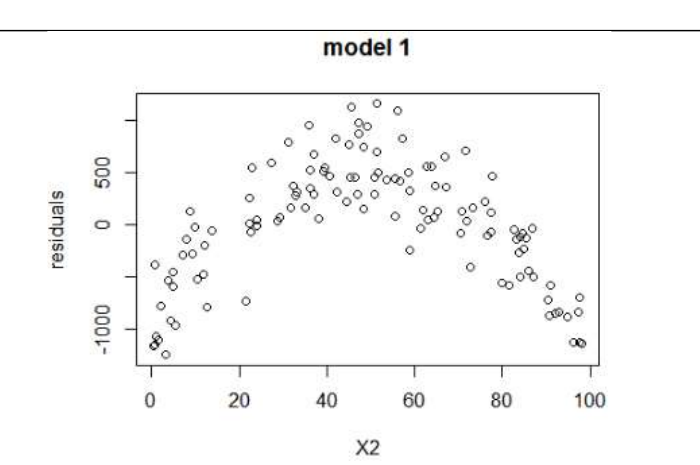
Real data from the exam: residuals of model (1) against X2 follow a clear inverted U.
(a) What does the snippet do? (b) What happens to the estimation results? (A) the intercept estimate will increase; (B) the standard error of will change; (C) the p-value of will not change; (D) none of the above. (c) Explain.
AI-written answer, not official. Check before relying on it.
a. What the code does [2 pts]
AnswerIt re-tests the coefficients of
ols1using heteroskedasticity-consistent (White, "HC0") robust standard errors:hccmcomputes the robust covariance matrix andcoeftestreports t-tests with it. The coefficient estimates are not re-estimated; only the SEs, t-values and p-values are recomputed.
b./c. Which statement is correct? [2 + 2 pts]
Answer: (B) the standard error of will changeJustification: robust SEs replace the usual formula with the White sandwich formula, so the standard errors (and therefore t-values and p-values) generally change, while the OLS coefficients stay exactly the same.
| Option | Verdict | Why |
|---|---|---|
| (A) intercept estimate will increase | Wrong | coeftest does not refit the model, so point estimates are identical. |
| (B) SE of will change | Correct | The SEs are recomputed with a different (robust) formula. |
| (C) p-value of will not change | Wrong | The p-value depends on the SE, which changes. (It may still print as below 2e-16 because the t-value is so large, but it is not guaranteed unchanged, so the statement is not true as a rule.) |
| (D) none of the above | Wrong | (B) holds. |
Low confidence(B) versus (C) hinges on the p-value of still being printed as
< 2e-16. The intended answer is (B): the exam wants "robust SEs change SEs but not coefficients".
IntuitionThe residual plot is an inverted U, a non-linear pattern in the mean (a missing term, see Q15), not a pattern in the variance. Robust SEs would fix SEs but cannot fix a misspecified functional form.
Background: Lec_12-Heteroskedasticity, Robust Standard Errors, White Correction.
Q14 — Residual vs random error [5 pts]
Question. What is the difference between a residual and a random error?
AI-written answer, not official. Check before relying on it.
Answer
- The random error is the deviation from the true population regression line. It is unobservable, because the true 's are unknown.
- The residual is the deviation from the estimated sample line. It is observable and is our estimate of the error.
Why it matters:
- By construction of OLS, residuals sum to zero and are uncorrelated with every regressor in the sample (when there is an intercept). The true errors need not do this in any given sample (they only satisfy it on average, under the exogeneity assumption).
- Residual variances differ across observations even when the errors are homoskedastic (high-leverage points have smaller residuals).
- Residuals are what we plot to diagnose the errors' assumptions (as in Q13).
Background: Residuals, Classical Assumptions, Lec_13-Exam Review (sections 1.1 and 1.2).
Q15 — Where is Y maximised? [5 pts]
Question. He adds : .
ols2   Y ~ X1and3 + X2 + X2.sq
              Estimate Std. Error t value Pr(>|t|)
(Intercept)   186.7853    81.3115   2.297    0.234
X1and3          1.8009     0.4272   4.215 4.96e-05 ***
X2             33.0327     3.3817   9.768  < 2e-16 ***
X2.sq          -0.6453     0.0338 -19.094  < 2e-16 ***
Residual standard error: 290.4 on 116 df
Multiple R-squared: 0.9234, Adjusted R-squared: 0.9214
F-statistic: 466.2 on 3 and 116 DF
At what value of is maximised?
AI-written answer, not official. Check before relying on it.
means an inverted U (a maximum, not a minimum). Differentiate with respect to (holding X1and3 fixed) and set to zero:
Answeris maximised at . This lies inside the observed range of X2 (0.05 to 97.9), so it is a meaningful peak, not an extrapolation. The sample's R² jumps from 0.68 (Q11) to 0.92 once the curvature is captured.
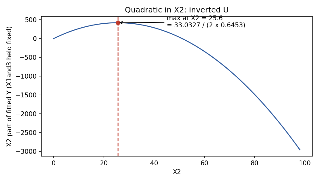
The X2 part of the fitted curve, , with its peak at (derived from the printed coefficients).
Printout quirkThe intercept row shows with p printed as 0.234. With 116 df, gives , so the printed p-value looks like a typo for 0.0234 (or the t value is mis-transcribed). See Q16.
Background: Quadratic Model, Lec_13-Exam Review (section 3.4), Assign_05-Quadratics, Dummy Variables, Interactions & the Chow Test.
Q16 — Dropping the intercept [10 pts]
Question. He notes the intercept in ols2 is not statistically significant and asks whether to omit it. (a) If , what can we say about the properties of in a model that omits the intercept? (b) If , what can we say about the properties of in model 2?
AI-written answer, not official. Check before relying on it.
a. and the intercept is omitted [5 pts]
Answeris biased and inconsistent. Forcing the line through the origin leaves out a relevant variable (the constant, with true coefficient ), which is omitted variable bias. The constant is correlated with regressors that have non-zero means (such as X2, mean about 51.8), so the slope absorbs part of the intercept's effect. The residuals also no longer sum to zero and the usual is not reliable.
b. and the intercept is kept [5 pts]
Answeris still unbiased and consistent, since including an irrelevant term does not bias OLS. It is, however, less efficient (larger variance) than the estimator from the model that correctly omits the intercept, because one extra parameter is estimated for nothing.
| Situation | Bias | Variance |
|---|---|---|
| Intercept omitted but | Biased | (smaller, but wrong target) |
| Intercept kept but | Unbiased | Larger (inefficient) |
IntuitionBetter too many than too few. A bit of extra variance is cheap; bias is not. So do not drop the intercept just because it is insignificant.
The premise is shakyThe exam says the intercept in
ols2is "not statistically significant", resting on the printed p-value 0.234. But with 116 df corresponds to , which is significant at 5%. The printed value looks like a typo, so the premise (and therefore the case for dropping the intercept) is weaker than the question suggests. The theory answers above do not depend on it.
Background: Regression Through the Origin, Omitted Variable Bias, Assign_03-Change of Variables, Regression Through the Origin & the Housing Model.
Q17 — Changing units of X2 and Y [5 pts]
Question. In model (2) we multiply by 2 and, at the same time, multiply by 3. What happens to all the coefficients, in terms of the model-2 coefficients?
AI-written answer, not official. Check before relying on it.
Define and (so ). Multiply the model by 3 and rewrite :
Answer
Coefficient New value Intercept (linear term) Rule: a coefficient is multiplied by (factor on Y) divided by (factor on its regressor). The squared term's regressor is scaled by . Standard errors scale the same way, so t-statistics, p-values, and F are unchanged.
Check with Q15: the new peak is , which is exactly twice the old peak, as it should be (the units of X2 doubled).
AssumptionThis assumes the squared term is recomputed from the rescaled variable (). If the squared variable were left in the old units, its coefficient would only be multiplied by 3.
Background: Change of Variables, Assign_03-Change of Variables, Regression Through the Origin & the Housing Model, Lec_13-Exam Review (section 3.1).
Recap
| Q | Topic | Tool | Answer (AI-written) |
|---|---|---|---|
| 1A | Group means | Dummy-variable reading | NA 2225.2; EU 389.3; AF 1196.8; AS 588.3 |
| 1B | EU = AS? | Linear restriction | |
| 2 | 99% vs 95% CI | p-value vs CI | TRUE (p = 0.031) |
| 3 | Date falls? | One-sided t | ; t = −1.20, fail to reject |
| 4 | WLS | Gauss-Markov | (C) unbiased and efficient |
| 5 | Day and date jointly | F-test | ; F ≈ 2.32 vs 2.01, reject (rounding-sensitive) |
| 6 | Marginal effect | Log-log | NIS per minute |
| 7 | Prediction | Interaction model | NIS |
| 8 | Bias in model 2 | Interactions, OVB | TRUE: 0.497 vs 0.221 for Europe |
| 9 | Continents | Chow test | ; df 3912; crit ≈ 1.49; F ≈ 5.16; reject |
| 10 | X1, X3 | Multicollinearity | High X1-X3 correlation; check corr/VIF |
| 11 | CI level | p-value | |
| 12 | anova |
F-test | ; fail to reject |
| 13 | coeftest(hc0) |
Robust SEs | (B) SE changes, coefficients do not |
| 14 | Residual vs error | Definitions | Estimated and observable vs true and unobservable |
| 15 | Peak | Quadratic | |
| 16 | No intercept | Omitted variable | : biased; : unbiased, inefficient |
| 17 | Units | Rescaling |
Related Notes
- Intro Econometrics (subject hub)
- Lec_13-Exam Review — covers the whole course, including the topics from lectures 1 to 7 that have no separate notes
- Lec_08-Goodness of Fit & Multicollinearity, Lec_10-Dummy Variables, Lec_11-Interaction Terms, Lec_12-Heteroskedasticity
- Assign_01-Interpreting OLS Output & the Birthweight-Smoking Regression, Assign_02-Functional Form & the Money-Supply Log-Log Model, Assign_03-Change of Variables, Regression Through the Origin & the Housing Model, Assign_05-Quadratics, Dummy Variables, Interactions & the Chow Test