
2024 Moed A — Antique Violins & Nonlinear X2 Models
- #intro-econometrics
- #past-paper
- #exam-prep
- #log-models
- #t-test
- #f-test
- #multicollinearity
- #r-squared
- #regression-through-origin
- #heteroskedasticity
- #dummy-variables
- #interaction-terms
- #quadratic
- #omitted-variable-bias
2024 Moed A — Antique Violins & Nonlinear X2 Models
Part of: Intro Econometrics Final Exam 2024 — Moed A (open notes, 3 hours, 100 points) — Introduction to Econometrics, Dr. Aluma Dembo Key concepts: Log-Level Model, Marginal Effect, Prediction, t-test, F-test, Hypothesis Testing, Confidence Interval, p-value, R-squared, Adjusted R-squared, Multicollinearity, Omitted Variable Bias, Regression Through the Origin, Heteroskedasticity, Gauss-Markov Theorem, Dummy Variable, Interaction Term, Quadratic Model Builds on: Lec_08-Goodness of Fit & Multicollinearity, Lec_10-Dummy Variables, Lec_11-Interaction Terms, Lec_12-Heteroskedasticity, Lec_13-Exam Review, Assign_02-Functional Form & the Money-Supply Log-Log Model, Assign_05-Quadratics, Dummy Variables, Interactions & the Chow Test
Full official keyThe instructor key (
Exam-2024-A-SOLUTIONS.pdf) answers all 15 questions. Every answer below follows it. Where the key's own arithmetic differs slightly from a recomputation, the answer is kept and a> [!warning]shows the check (Q2, Q11, Q13). No question was AI-solved. Items marked> [!tip] Intuitionare added explanation, not part of the key.
Date conflict in the headerThe cover page says "2024 - Moed A" but also "February 15, 2023 at 15:45". The title (2024 Moed A) is used here; the 2023 date looks like a leftover from the previous year's template.
Format100 points, open notes. Part A is Q1 to Q8 (violins, 49 points). Part B is Q9 to Q15 (anonymous X1, X2, X3 and Y, N = 117; 51 points). Each multiple-choice or T/F item needs a short justification in the exam, so every answer below gives the justification and says why the other options fail.
What this paper tests
- Part A: read t-test / F-test output (one-sided test, joint goodness of fit, a linear-restriction F test), predictions and marginal effects in a Log-Level Model, why dropping a variable can lower Adjusted R-squared (Multicollinearity), dropping the intercept, and spotting Heteroskedasticity in a residual plot.
- Part B: confidence intervals vs p-values, a joint F test that replaces a linear term by two dummies, dummies plus interactions (piecewise lines), a Quadratic Model and its maximum, matching estimated models to pictures, and when a variable is irrelevant.
IntuitionAlmost every question is "find the right row of R output". Decide first which test the question wants (single coefficient: t; several at once or the whole model: F), then read the number off the printout.
Part A — Antique violins as an investment
Data: 222 antique violin sales. Variables: ln_sale_price (log sale price, 2005 GBP), saleyear, yearbuilt, stradivari (=1 if made by Antonio Stradivari), is_named (=1 if the violin has a name). The scatter in the paper shows log price rising with sale year, from about 5 to 6 around 1860 to about 10 to 15 by 2000.
Q1 — One-sided t test on sale year [5 pts]
Model (1):
R output for sales1 (n = 222, 217 df):
| Variable | Estimate | Std. Error | t value | Pr(>|t|) |
|---|---|---|---|---|
| (Intercept) | -1.049e+02 | 5.159e+00 | -20.330 | < 2e-16 |
| saleyear | 5.753e-02 | 2.094e-03 | 27.474 | < 2e-16 |
| yearbuilt | 3.320e-04 | 1.627e-03 | 0.204 | 0.838 |
| stradivari | 3.810e-01 | 2.070e-01 | 1.841 | 0.067 |
| is_named | 1.518e+00 | 2.370e-01 | 6.405 | 9.21e-10 |
Residual SE 1.088 on 217 df; R² = 0.7847, adjusted R² = 0.7807; F = 197.7 on 4 and 217 df, p < 2.2e-16.
a. Null hypothesis [2 pts]
Official answer(the alternative is ).
The researcher believes price increases with saleyear, so the claim to establish goes in and "no increase" is the null.
b. Critical value at 5% [2 pts]
Official answer1.645, a one-tailed test with 217 degrees of freedom.
Exact valueThe exact one-sided 5% value is about 1.652; 1.645 is the normal approximation, and the key uses it. The conclusion is identical either way.
c. Conclusion [1 pt]
Official answerReject at 5%. The test statistic is , far above 1.645.
Because the p-value printed is two-sided, you can also halve it: the one-sided p is below .
Q2 — Predicted sale price [5 pts]
Unnamed () Stradivari (), built 1736, sold 1867.
Official answer30.175 GBP (2005 prices).
The model predicts the log price, so you must exponentiate to get a price. The key notes that answers differing because of rounding are accepted.
Rounding sensitivityPlugging the printed 4-digit coefficients straight in gives and a price of about 32.0, not 30.175. The gap is rounding: the printed
saleyearcoefficient is multiplied by 1867, so a change in its 5th digit moves the answer by about 0.001 per 0.0000005, and the intercept is printed to only 4 significant figures (-1.049e+02). The key's 3.407 uses unrounded estimates. Keep the official 30.175 and expect "about 30 to 32" to be accepted.
Q3 — Marginal effect of sale year on the price [5 pts]
The exam supplies summary(sales1$model) (the means of the variables): mean ln_sale_price = 9.660, mean saleyear = 1959, mean yearbuilt = 1728, mean stradivari = 0.5676, mean is_named = 0.7162.
Official answer901.9 (or 0.556, depending on whether the price or the log price is used).
In a log-level model the effect on the level of price is
evaluated at the average price:
Interpretation: holding build year, maker and fame fixed, waiting one more year to sell raises the price by about 902 GBP on average, evaluated at the typical (mean log) price.
Mistake in the question, acknowledged by the keyThe question does not give the average sale price, only the average of the log price. The key says answers using 9.66 or get full credit. Using 9.66 directly gives (not meaningful as a price effect, but accepted).
Intuitionalso reads as "each extra year of waiting raises the price by about 5.75%" (log-level rule). The marginal effect in GBP is that percentage times the price level, which is why it depends on the price.
Q4 — Why does adjusted R² fall when stradivari is dropped? [7 pts]
Model (2) drops stradivari, model (3) drops is_named.
| Model (1) all four | Model (2) no stradivari | Model (3) no is_named | |
|---|---|---|---|
| saleyear | 0.05753 (t 27.474) | 0.05689 (t 27.398) | 0.053349 (t 24.647) |
| yearbuilt | 0.000332 (p 0.838) | -0.0001884 (p 0.907) | -0.001677 (p 0.335) |
| stradivari | 0.3810, SE 0.2070, p 0.067 | dropped | 1.091748, SE 0.190087, p 3.09e-08 |
| is_named | 1.518, SE 0.2370, p 9.21e-10 | 1.752, SE 0.2011, p 7.73e-16 | dropped |
| R² | 0.7847 | 0.7813 | 0.744 |
| Adjusted R² | 0.7807 | 0.7783 | 0.7405 |
| Residual SE (df) | 1.088 (217) | 1.094 (218) | 1.184 (218) |
a. What explains it? [4 pts]
Official answer
stradivariandis.namedare probably highly correlated. Including both in model (1) creates partial Multicollinearity, which inflates the standard error ofstradivariand makes it look insignificant (p = 0.067). Butstradivaridoes affect price: whenis.namedis dropped instead (model 3),stradivariis highly significant (p = 3.09e-08). So removing it from model (1) loses real explanatory power and the adjusted R² falls (0.7807 to 0.7783).
How to see it in the output: the stradivari coefficient is 0.381 next to is_named but 1.092 alone, because with both present they share the same effect. That is the signature of overlapping regressors.
IntuitionAdjusted R² rises when you drop a regressor only if its |t| is below 1. Here the
stradivarit is 1.841, above 1 although below the 5% cutoff of about 1.97. So "insignificant at 5%" does not mean "adjusted R² improves when removed": the variable still carries information.
b. Code to check [3 pts]
Official answerCheck the correlation between the two dummies:
cor(violin$stradivari, violin$is.named)Also accepted: their covariance, or a regression of
stradivarionis.named.
(The key's printed code spells the variable stradivary; the variable in the data is stradivari.)
Q5 — Goodness of fit for model (4) [7 pts]
Model (4), now with the log return on investment as outcome (ln_ROI = log of sale price / purchase price):
| Variable | Estimate | Std. Error | t value | Pr(>|t|) |
|---|---|---|---|---|
| (Intercept) | -2.016e+01 | 5.014e+00 | -4.020 | 8.03e-05 |
| saleyear | 6.252e-02 | 2.645e-03 | 23.635 | < 2e-16 |
| purchaseyear | -5.141e-02 | 2.759e-03 | -18.635 | < 2e-16 |
| yearbuilt | -7.403e-04 | 1.498e-03 | -0.494 | 0.622 |
| is_named | 1.709e-01 | 2.090e-01 | 0.818 | 0.414 |
Residual SE 1.017 on 217 df; R² = 0.731, adjusted R² = 0.7261; F = 147.4 on 4 and 217 df, p < 2.2e-16.
a. Select one [2 pts]
Official answer(C) The model is a good fit because the p-value on the F-statistic is smaller than 0.05.
- (A) wrong: it reasons from individual p-values and lists , but a goodness-of-fit test is a joint test, not a list of single t tests.
- (B) wrong: same mistake in the other direction. Two insignificant coefficients ( and ) do not make the model a bad fit.
- (D) wrong: (C) is correct.
b. Explanation [5 pts]
Official answerThe F statistic on the last line tests (all slope coefficients are zero, so the regressors jointly explain nothing). It is a joint null, so the individual p-values in the last column cannot be used. The F p-value is below 0.05, so we reject : the model is a good fit.
Q6 — Dropping the intercept [5 pts]
Model (5) replaces saleyear and purchaseyear by holding.period = saleyear - purchaseyear:
| Model (5), with intercept | Estimate | Std. Error | t value | Pr(>|t|) |
|---|---|---|---|---|
| (Intercept) | 1.8683149 | 2.7895826 | 0.670 | 0.5037 |
| holding_period | 0.0576974 | 0.0026168 | 22.049 | <2e-16 |
| yearbuilt | -0.0007488 | 0.0015836 | -0.473 | 0.6368 |
| is_named | -0.4584016 | 0.1795233 | -2.553 | 0.0113 |
R² = 0.6979, adjusted R² = 0.6938, residual SE 1.075 on 218 df.
| Model (6), no intercept | Estimate | Std. Error | t value | Pr(>|t|) |
|---|---|---|---|---|
| holding_period | 5.778e-02 | 2.611e-03 | 22.133 | < 2e-16 |
| yearbuilt | 3.103e-04 | 8.187e-05 | 3.791 | 0.000194 |
| is_named | -4.109e-01 | 1.647e-01 | -2.494 | 0.013353 |
R² = 0.8622, adjusted R² = 0.8603, residual SE 1.074 on 219 df.
Official answerWhen the intercept is omitted, increases (from -0.000749 to +0.000310) and becomes statistically significant (p from 0.637 to 0.0002). That means the intercept was probably not truly zero: leaving out a non-zero intercept biases the other coefficients (and so they are not efficient/reliable). If the true intercept were zero, model (6) would only omit an irrelevant variable and the other estimates would not change much. The researcher should use model (5).
Do not compare the R² valuesR² jumps from 0.698 to 0.862 in model (6), but that is not an improvement. Without an intercept R² may be computed around zero instead of around the mean of , so it is not comparable with a regression that has an intercept. The R² rise is an artefact, not evidence for model (6). See Regression Through the Origin and Assign_03-Change of Variables, Regression Through the Origin & the Housing Model.
Q7 — F test comparing models (4) and (5) [8 pts]
> anova(roi4, roi5)
  Res.Df    RSS Df Sum of Sq      F    Pr(>F)
1    217 224.30
2    218 251.88 -1   -27.582 26.684 5.417e-07 ***
Model 1 = roi4 (saleyear, purchaseyear, yearbuilt, is_named). Model 2 = roi5 (holding_period, yearbuilt, is_named).
a. Null hypothesis [3 pts]
Official answerOn model (4): , equivalently .
b. Unrestricted vs restricted [3 pts]
Official answerModel (4) is unrestricted; model (5) is restricted. Imposing on model (4) turns it into model (5):
The restriction is that sale year and purchase year enter with equal and opposite coefficients, i.e. only the gap between them (the holding period) matters.
c. Conclusion [2 pts]
Official answerReject at 5%: the F p-value (5.417e-07) is far below 0.05.
Check: , matching the output. The restricted model fits significantly worse, so holding period alone is not enough: sale year and purchase year have effects that are not exactly equal and opposite (0.0625 vs -0.0514 in model 4).
Q8 — Residuals against sale year [7 pts]
The residuals of model (4) are plotted against saleyear (real data in the paper): they have a small, tight spread for sale years before about 1950, and a much wider spread (roughly -2 to +4) after about 1975, i.e. the variance grows with the sale year. (The statements refer to "ols1", the paper's name for the model being plotted.)
a. Select one [2 pts]
Official answer(C) Both (A) and (B) are reasonable statements.
- (A) The estimate of is not efficient: true. The pattern signals Heteroskedasticity, so assumption A4 (constant variance) fails; the Gauss-Markov theorem no longer applies and OLS is no longer BLUE / efficient.
- (B) The standard error of is biased: true. The usual formula for the standard error assumes constant variance, so under heteroskedasticity it is biased (and t tests are unreliable).
- (D) wrong: both statements hold.
Note the estimate itself is still unbiased; only efficiency and the standard errors are affected.
b. Explain, naming the issue [5 pts]
Official answerThe plot shows model (4) likely has heteroskedasticity: is a function of
saleyearand is not constant. Because A4 is violated, Gauss-Markov no longer holds and the OLS estimates cannot be concluded to be efficient, so (A) is true. Under heteroskedasticity the standard errors are biased, so (B) is also reasonable. Hence (C).
IntuitionFix: use heteroskedasticity-robust (White) standard errors, or weighted least squares. See Lec_12-Heteroskedasticity. The residual cloud also sags in the middle (below zero around 1950) and rises again, which can additionally hint at a non-linear trend in
saleyear. The key names only heteroskedasticity.
Part B — A colleague's model (X1, X2, X3 and Y)
Data: N = 117 independent random observations, summary statistics below. Summary of the variables:
| Min | 1st Qu. | Median | Mean | 3rd Qu. | Max | |
|---|---|---|---|---|---|---|
| Y | -1140.3 | 511.3 | 1007.8 | 891.3 | 1369.2 | 2245.0 |
| X1 | 0.2268 | 20.5557 | 51.0561 | 49.5389 | 76.1373 | 98.3967 |
| X2 | 0.8196 | 23.6742 | 50.0388 | 50.2647 | 75.8186 | 99.8334 |
| X3 | -3.14260 | -0.79117 | -0.11350 | -0.09998 | 0.69459 | 2.74763 |
Base model (1):
| ols1 | Estimate | Std. Error | t value | Pr(>|t|) |
|---|---|---|---|---|
| (Intercept) | 989.918 | 150.943 | 6.558 | 1.70e-09 |
| X1 | 6.765 | 2.024 | 3.342 | 0.00113 |
| X2 | -8.519 | 2.080 | -4.096 | 7.92e-05 |
| X3 | 56.108 | 57.413 | 0.977 | 0.33052 |
Residual SE 668.2 on 113 df; R² = 0.1892, adjusted R² = 0.1677; F = 8.79 on 3 and 113 df, p = 2.744e-05.
Q9 — 99% and 90% confidence intervals for X3 [5 pts]
Claim: the 99% CI for the X3 coefficient includes 0 but the 90% CI does not.
Official answerFALSE.
The p-value of is 0.33. A confidence interval excludes 0 only if the p-value is below . Since is above both 0.01 and 0.10, neither interval excludes 0. (In the key's words, the confidence intervals from about 67% upwards include zero.) So the 99% interval includes zero, and so does the narrower 90% interval, and the claim that the 90% interval excludes zero is false.
IntuitionHigher confidence means a wider interval. If the wider one (99%) contains 0 the narrower one (90%) may or may not. Here the 90% one also contains 0, so the claim fails. For the claim to be true you would need .
Q10 — Dummies for low and high X2: joint F test [8 pts]
Model (2): , with X2.is.L = 1 if X2 < 25 and X2.is.H = 1 if X2 > 75.
| ols2 | Estimate | Std. Error | t value | Pr(>|t|) |
|---|---|---|---|---|
| (Intercept) | 1082.201 | 92.569 | 11.691 | < 2e-16 |
| X1 | 6.663 | 1.391 | 4.791 | 5.13e-06 |
| X2.is.L | -651.720 | 103.350 | -6.306 | 5.86e-09 |
| X2.is.H | -1305.040 | 103.489 | -12.610 | < 2e-16 |
| X3 | 25.468 | 39.540 | 0.644 | 0.521 |
R² = 0.6203, adjusted R² = 0.6068, residual SE 459.3 on 112 df.
The anova(ols2.restr, ols2) output (the restricted formula is blacked out in the paper):
  Res.Df      RSS Df Sum of Sq      F  Pr(>F)
1    114 57950055
2    112 23627617  2  34322438 81.348 < 2.2e-16 ***
a. Null hypothesis [3 pts]
Official answer(the low and high dummies do not matter, so no non-linearity of this kind).
b. Restricted model [2 pts]
Official answer. (The key notes the index on the X3 coefficient does not matter.)
This is the model with both dummies removed; note it has 114 residual df, 2 more than the unrestricted 112, matching the 2 restrictions. It does not contain a linear X2 term, so the test asks whether these two dummies add anything, as a stand-in for non-linearity.
c. Conclusion [3 pts]
Official answerReject at 5%: with p-value < 2.2e-16, far below 0.05. We conclude there is a nonlinear relationship between X2 and Y.
Check: .
Q11 — Predicted Y from model (3) [9 pts]
Model (3) adds the interactions X2.L.interact = X2.is.L × X2 and X2.H.interact = X2.is.H × X2, and keeps a plain X2 term:
| ols3 | Estimate | Std. Error | t value | Pr(>|t|) |
|---|---|---|---|---|
| (Intercept) | 1640.2766 | 161.7302 | 10.142 | < 2e-16 |
| X1 | 6.5211 | 0.9941 | 6.560 | 1.87e-09 |
| X2.is.L | -1791.9920 | 194.1924 | -9.228 | 2.47e-15 |
| X2.L.interact | 59.9984 | 8.7706 | 6.841 | 4.79e-10 |
| X2.is.H | 3931.1090 | 764.9824 | 5.139 | 1.22e-06 |
| X2.H.interact | -55.3324 | 9.0225 | -6.133 | 1.41e-08 |
| X2 | -10.8413 | 2.9333 | -3.696 | 0.000345 |
| X3 | 7.8439 | 28.7813 | 0.273 | 0.785727 |
R² = 0.8116, adjusted R² = 0.7995, residual SE 328 on 109 df; F = 67.08 on 7 and 109 df.
Official answer831.28 when X2 = 20, 1098.27 when X2 = 50, 277.78 when X2 = 80.
With X1 = X3 = 0, only the intercept, the dummies and X2 remain:
Working
- X2 = 50 (middle): both dummies are 0, so both interactions are 0. .
- X2 = 20 (low):
X2.is.L= 1,X2.L.interact= 20,X2.is.H= 0. .- X2 = 80 (high):
X2.is.H= 1,X2.H.interact= 80,X2.is.L= 0. .
Rounding in the keyWith all the printed digits I get 831.43, 1098.21 and 277.49. The key rounds the slopes to two decimals (49.15, -10.84, -66.17) before multiplying, which shifts the answers by 0.06 to 0.3. These are rounding differences; keep the official values (the exam allows 3 significant figures).
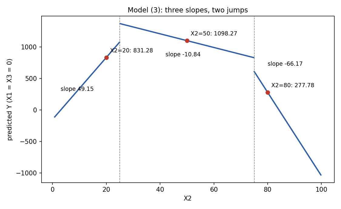
Model (3) drawn from the printed coefficients (X1 = X3 = 0), with the three predictions marked. Slopes and predicted values are the key's.
Q12 — Marginal effect of X2 in model (3) [9 pts]
Official answer49.15 when X2 < 25; -10.84 when 25 < X2 < 75; -66.17 when X2 > 75.
Differentiate with respect to X2 and switch the dummies on and off:
Working
- Between 25 and 75: both dummies are 0, so the interactions vanish and the marginal effect is just .
- Below 25:
X2.is.L= 1, soX2.L.interact= X2 and the effect is .- Above 75:
X2.is.H= 1, soX2.H.interact= X2 and the effect is .
Each extra unit of X2 raises Y by 49.15 in the low region, lowers it by 10.84 in the middle and by 66.17 at the top. The dummies and shift the level (the jumps in the picture); the interactions change the slope. See Lec_11-Interaction Terms.
Q13 — X2 that maximises predicted Y in model (4) [5 pts]
| ols4 | Estimate | Std. Error | t value | Pr(>|t|) |
|---|---|---|---|---|
| (Intercept) | -224.93004 | 90.26631 | -2.492 | 0.0142 |
| X1 | 6.44078 | 0.92275 | 6.980 | 2.21e-10 |
| X2 | 69.24973 | 3.85954 | 17.942 | < 2e-16 |
| X2.sq | -0.78464 | 0.03775 | -20.786 | < 2e-16 |
| X3 | 23.70234 | 26.21168 | 0.904 | 0.3678 |
R² = 0.8331, adjusted R² = 0.8271, residual SE 304.5 on 112 df; F = 139.8 on 4 and 112 df.
Official answerX2 = 44.11.
Working.
Since the parabola opens downward, so this stationary point is a maximum.
Rounding in the keyWith the unrounded coefficients . The key's 44.11 comes from rounding the coefficients to 69.25 and 0.785. Both round to about 44, and the exam allows rounding.
Intuition44.11 lies between 25 and 75, which agrees with the model (3) picture where the slope turns negative after the low region. A maximum inside the data range (X2 runs 0.8 to 99.8) is a sensible turning point; one outside the range would not be.
Q14 — Which plot matches which model? [8 pts]
The four plots (drawn in the paper): NW a straight falling line; NE a rising line, a jump up at 25, a gently falling line to 75, a jump down at 75, then a steeply falling line; SW three flat segments (low, high, lowest); SE an upside-down parabola.
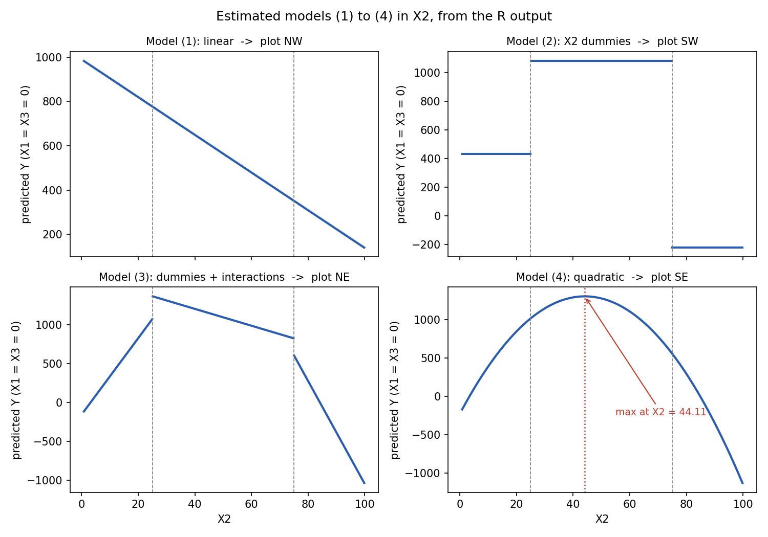
The four estimated models plotted from the printed coefficients (X1 = X3 = 0). The plot labels match the key; the shapes are the estimated ones.
a. Model (1)
Official answerPlot NW. Model (1) is linear in X2 with an estimated negative slope (-8.519), and NW is a straight falling line.
b. Model (2)
Official answerPlot SW. Model (2) is a step function: level below 25, between 25 and 75, above 75. With and the middle level is highest and the top is lowest, which is SW.
c. Model (3)
Official answerPlot NE. Model (3) has a different intercept and slope in each region: slope 49.15 below 25, -10.84 between 25 and 75, -66.17 above 75, with jumps at 25 and 75 (the dummies).
d. Model (4)
Official answerPlot SE. Model (4) is quadratic with a negative squared term, so an upside-down parabola with its maximum at X2 = 44.11.
Q15 — Is X3 an irrelevant variable? [7 pts]
Model (5) of Part B (called ols5) drops X3 from model (4):
| ols5 | Estimate | Std. Error | t value | Pr(>|t|) |
|---|---|---|---|---|
| (Intercept) | -229.07144 | 90.07731 | -2.543 | 0.0123 |
| X1 | 6.41541 | 0.92158 | 6.961 | 2.35e-10 |
| X2 | 69.44801 | 3.85020 | 18.038 | < 2e-16 |
| X2.sq | -0.78667 | 0.03765 | -20.894 | < 2e-16 |
R² = 0.8319, adjusted R² = 0.8274, residual SE 304.3 on 113 df; F = 186.4 on 3 and 113 df.
a. Select one [2 pts]
Official answer(B) Yes, the estimated coefficient on X3 in model (4) is not statistically significant.
- (A) wrong: "omitting X3 biases the X1 coefficient". Dropping X3 barely changes the other estimates (X1: 6.441 to 6.415; X2: 69.25 to 69.45; X2.sq: -0.785 to -0.787; intercept -224.9 to -229.1), so there is no evidence of bias.
- (C) wrong: it reasons from R² falling "from 8.331 to 8.319" (a typo for 0.8331 to 0.8319). R² cannot be used to compare models with different numbers of regressors, because it never falls when you add a variable. The right comparison is adjusted R².
- (D) wrong: (B) is correct.
b. Explain [5 pts]
Official answerThe answer is (B) because the p-value of the X3 coefficient in model (4) is 0.38 (the printed value is 0.3678), much greater than 5%, so it is not statistically different from zero. (A) is incorrect because the other coefficients do not change much when X3 is omitted in
ols5. (C) is incorrect because R² cannot be used to compare models with different numbers of explanatory variables; use adjusted R² instead.Also acceptable per the key: arguing (D) on the grounds that the adjusted R² goes up (0.8271 to 0.8274). If a student argues that the coefficients are different, indicating bias, argument (A) would also be accepted.
Recap table
| Q | Topic | Tool | Official answer |
|---|---|---|---|
| 1 | Sale price rises over time? | One-sided t test | ; crit 1.645; t = 27.47; reject |
| 2 | Prediction, unnamed Stradivari 1736/1867 | Exponentiate log prediction | GBP |
| 3 | Marginal effect of saleyear | price | 901.9 (or 0.556) |
| 4 | Adjusted R² falls when stradivari dropped | Multicollinearity | stradivari and is.named correlated; check with cor() |
| 5 | Goodness of fit, model (4) | F test, joint | (C); : all slopes = 0; reject |
| 6 | Drop the intercept | Omitted intercept | rises and turns significant; use model (5) |
| 7 | anova(roi4, roi5) | F test of | (4) unrestricted, (5) restricted; reject |
| 8 | Residuals vs saleyear | Heteroskedasticity | (C); not efficient, SE biased |
| 9 | CI claim for X3 | p = 0.33 | FALSE |
| 10 | Dummies for low/high X2 | Joint F test | ; reject; nonlinear |
| 11 | Model (3) predictions | Dummies and interactions | 831.28, 1098.27, 277.78 |
| 12 | Marginal effect in model (3) | Slope by region | 49.15, -10.84, -66.17 |
| 13 | Max of quadratic | 44.11 | |
| 14 | Plots vs models | Shapes | NW, SW, NE, SE |
| 15 | Is X3 irrelevant? | t test, coefficient stability | (B) |
Related notes
- Intro Econometrics (hub)
- Lec_08-Goodness of Fit & Multicollinearity, Lec_10-Dummy Variables, Lec_11-Interaction Terms, Lec_12-Heteroskedasticity, Lec_13-Exam Review
- Assign_01-Interpreting OLS Output & the Birthweight-Smoking Regression, Assign_02-Functional Form & the Money-Supply Log-Log Model, Assign_03-Change of Variables, Regression Through the Origin & the Housing Model, Assign_05-Quadratics, Dummy Variables, Interactions & the Chow Test