
Lecture 7 — NLP & Image Analysis: Making Sense of Words and Pictures
- #data-science
- #intro-data-science
- #nlp
- #text-preprocessing
- #bag-of-words
- #document-term-matrix
- #tf-idf
- #image-analysis
- #computer-vision
- #convolution
- #filters
- #unstructured-data
Lecture 7 — NLP & Image Analysis
Part of: Data Science Previous: Lecture 6 - Recommendation Systems | Next: Lecture 8 - Intro to Deep Learning Key concepts: Unstructured Data, NLP, Text Preprocessing, Tokenization, Stopwords, Stemming, Lemmatization, Bag-of-Words, Document-Term Matrix, TF-IDF, Cosine Similarity, Pixel, Convolution, Filter, Feature Map, CNN
The Core Idea
Lectures 3 to 6 only worked on numeric tables. Most real data is not: emails, reviews, support tickets, photos, scans. This lecture is about the translation step: turning text and images into a numeric feature matrix, so that the models you already know (classifiers, K-Means, recommenders) can be applied unchanged.
One-line summaryUnstructured data → preprocessing → numeric features → models from Lectures 3 to 6. NLP and image analysis are feature engineering for non-numeric data.
The 80% problemThe deck quotes the estimate that about 80% of business data is unstructured (emails, reviews, tickets, social posts, photos, video, PDFs, chat logs). The DataFrames of Lectures 2 to 6 are the other 20%.
Running case: Bikoret, a (fictional) Tel Aviv restaurant-review platform with 30 restaurants, 300 reviews and many food photos. The Head of Product, Shira, sees star ratings but cannot read 300 reviews. Her question: what are customers SAYING (text) and SHOWING (photos)?
Why stars are not enoughA 3-star review can mean "decent food, decent service" or "amazing food, awful waiter" (food 5/5, service 1/5). The star averages the two into one number and hides the real signal. The same logic: 500 reviews averaging 3.5 could be 300 "incredible food" and 200 "worst service ever".
| Text (NLP) | Images (Computer Vision) | |
|---|---|---|
| Raw form | A sequence of words | A grid of pixel numbers |
| Challenge | Meaning, context, ambiguity, sarcasm, synonyms | A "cat" looks different in every photo (pose, light, background) |
| Conversion problem | Needs a pipeline to become numbers | Already numbers; the problem is extracting useful features |
| Feature tool | Bag-of-Words counts | Filter responses (Convolution) |
Part A — Text (NLP)
NLP (Natural Language Processing) is the field of AI concerned with letting computers understand, interpret and generate human language (as opposed to programming languages). It powers chatbots, spam filters, auto-complete, translation, sentiment analysis, topic detection, summarisation and voice assistants.
The text preprocessing pipeline
Raw text → lowercase → remove punctuation → tokenize → remove stopwords → stem/lemmatize → clean tokens
Think of it as an assembly line: messy text goes in, a tidy list of meaningful words comes out. Every NLP system, from spam detection to ChatGPT, starts with some version of this.
| Step | What it does | Why | Example |
|---|---|---|---|
| Lowercase | The → the |
String comparison is case-sensitive, so Food and food would count as different words |
"Best shakshuka in Tel Aviv" → "best shakshuka in tel aviv" |
| Remove punctuation | strip , . ! |
amazing, amazing!, amazing, would be three different strings |
"terrible service, waited…" → "terrible service waited…" |
| Tokenization | sentence → list of words (tokens) | Creates countable, discrete units | "the hummus was absolutely amazing and fresh" → 7 tokens |
| Stopwords removal | drop the, is, at, was, a, and, for, in, of, to, but… |
Focuses on content words; typically cuts token count by 40 to 60% | 7 tokens → hummus, absolutely, amazing, fresh |
| Stemming / Lemmatization | reduce word variants to one form | Groups prices/price, waited/wait |
see below |
Pitfalls of each step
- Lowercasing loses information:
Apple(company) becomesapple(fruit). For most business NLP the trade-off is worth it.- Stopword removal can destroy negation.
notis often a stopword, yet "not good" means the opposite of "good". This is a known limitation for Bag-of-Words.- Simple tokenizing splits on spaces; better tokenizers also handle contractions (
don't→do+not), hyphens and special characters.
Stemming vs lemmatization
Stemming chops suffixes by rule; the stem may not be a real word. Lemmatization uses a vocabulary and grammar to return the true dictionary form (the lemma).
| Original | Stem (rough) | Lemma (correct) |
|---|---|---|
| amazing | amaz | amazing |
| waited | wait | wait |
| ingredients | ingredi | ingredient |
| better | better | good |
| running | run | run |
| beautiful | beauti | beautiful |
| Stemming | Lemmatization | |
|---|---|---|
| Speed | Fast (chop suffixes) | Slower (dictionary lookup) |
| Output | May not be real words | Always real words |
| Accuracy | Good enough for most tasks | Better for precise analysis |
| Use when | Speed matters, large datasets | Accuracy matters, smaller datasets |
| Tools | Porter Stemmer, Snowball | WordNet Lemmatizer, spaCy |
Rule of thumbStemming is faster, lemmatization is smarter; for sentiment or topic work the difference is small. Pick one and be consistent. Bikoret uses lemmatization because the corpus is small and Shira wants readable output.
Worked example: the 8 demo reviews
| ID | Original | Cleaned tokens | # |
|---|---|---|---|
| R1 | The hummus was absolutely amazing and fresh | hummus, absolutely, amazing, fresh | 4 |
| R2 | Terrible service, waited forty minutes for a menu | terrible, service, wait, forty, minute, menu | 6 |
| R3 | Great food but the restaurant was too noisy | great, food, restaurant, noisy | 4 |
| R4 | Best shakshuka in Tel Aviv, highly recommend | best, shakshuka, tel, aviv, highly, recommend | 6 |
| R5 | The prices are way too high for small portions | price, way, high, small, portion | 5 |
| R6 | Beautiful rooftop setting with amazing views | beautiful, rooftop, setting, amazing, view | 5 |
| R7 | The food was not good and the waiter was rude | food, good, waiter, rude | 4 |
| R8 | Fresh ingredients, reasonable prices, friendly staff | fresh, ingredient, reasonable, price, friendly, staff | 6 |
Note R7: not has been dropped, so a negative review now reads "food good waiter rude".
Python: the pipeline in code
Not from the slidesThe deck has no code. The snippet below is my own illustration of the steps (run and checked; see the caveat on stopword lists after it).
import string
from sklearn.feature_extraction.text import ENGLISH_STOP_WORDS

def preprocess(text):
    text = text.lower()                                              # 1. lowercase
    text = text.translate(str.maketrans("", "", string.punctuation))  # 2. strip punctuation
    tokens = text.split()                                            # 3. tokenize on spaces
    return [w for w in tokens if w not in ENGLISH_STOP_WORDS]        # 4. drop stopwords

preprocess("Terrible service, waited forty minutes for a menu")
# ['terrible', 'service', 'waited', 'minutes', 'menu']
Step 5 (lemmatize) would turn waited → wait and minutes → minute; in practice use nltk.WordNetLemmatizer or spaCy. Different libraries ship different stopword lists: scikit-learn's list also removes forty and not, whereas the slides' hand-worked version keeps forty, so counts can differ slightly from the slides.
Exploring the Bikoret data
Two tables: reviews.csv (300 rows: review_id, restaurant_id (join key), reviewer_name, review_text (the NLP input), rating, category (topic label)) and restaurants.csv (30 rows).
| Quick EDA fact | Value |
|---|---|
| Reviews / restaurants | 300 / 30 (about 10 reviews per restaurant) |
| Rating mean / mode | about 3.6 / 4 |
| Category split | Food 40%, Service 25%, Ambiance 20%, Price 15% |
| Review length | about 12 words raw, about 6 cleaned |
25% of reviews are about service: signal the star rating alone misses.
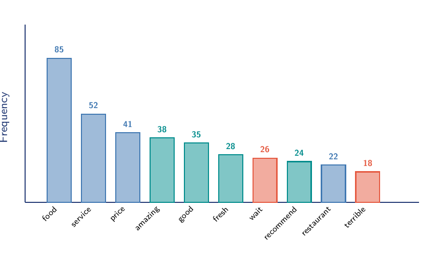
Top word counts after cleaning (from the slides): food 85, service 52, price 41, amazing 38, good 35, fresh 28, wait 26, recommend 24, restaurant 22, terrible 18, then noisy 15, friendly 14, view 12, portion 11, rude 10.
Frequency is not importance"Food" appears 85 times but in both positive and negative reviews. A rare word that appears only in negative reviews (like
rude) can be more informative. This motivates TF-IDF below.
Bag-of-Words and the document-term matrix
Bag-of-Words (BoW) describes each document as a vector of word counts; word order is thrown away ("The food was great" and "Great was the food" give the same bag).
Steps for review R1:
- Cleaned tokens:
hummus, absolutely, amazing, fresh. - Vocabulary = all unique words across all reviews (about 38 in the demo).
- Count each vocabulary word in R1 (1 for
absolutely,amazing,fresh,hummus; 0 for the rest). - R1's vector is mostly zeros with four 1s.
Stacking these vectors gives the Document-Term Matrix (DTM): rows = documents, columns = terms, values = counts.
| amazing | best | food | fresh | good | hummus | noisy | price | recommend | rude | service | terrible | |
|---|---|---|---|---|---|---|---|---|---|---|---|---|
| R1 | 1 | 0 | 0 | 1 | 0 | 1 | 0 | 0 | 0 | 0 | 0 | 0 |
| R2 | 0 | 0 | 0 | 0 | 0 | 0 | 0 | 0 | 0 | 0 | 1 | 1 |
| R3 | 0 | 0 | 1 | 0 | 0 | 0 | 1 | 0 | 0 | 0 | 0 | 0 |
| R4 | 0 | 1 | 0 | 0 | 0 | 0 | 0 | 0 | 1 | 0 | 0 | 0 |
| R5 | 0 | 0 | 0 | 0 | 0 | 0 | 0 | 1 | 0 | 0 | 0 | 0 |
| R6 | 1 | 0 | 0 | 0 | 0 | 0 | 0 | 0 | 0 | 0 | 0 | 0 |
(12 of the about 38 columns, rows R1 to R6, as on the slide.)
The bridgeThe DTM is a feature matrix, exactly like the ones from Lectures 3 to 5: each word is a feature, each review a data point. That is why every earlier technique now applies.
from sklearn.feature_extraction.text import CountVectorizer

vectorizer = CountVectorizer()                   # builds the vocabulary and counts words
dtm = vectorizer.fit_transform(cleaned_reviews)  # sparse matrix: documents x terms
print(dtm.shape)                                 # (n_reviews, vocabulary_size)
print(vectorizer.get_feature_names_out())        # the column (term) names
Not from the slides
CountVectorizeris the standard scikit-learn tool for this; I ran it on three of the demo reviews and got a(3, 13)matrix.cleaned_reviewsis a list of space-joined cleaned strings.
Reconstructed from the slides: shape of a DTMA corpus of reviews with vocabulary size gives an matrix. Examples from the exercises: 1,000 reviews and 800 unique words give a DTM; 5,000 reviews and a 2,000-word vocabulary give .
Sparsity (again)
Most DTM entries are 0: a short review uses 4 to 6 of about 38 words, so each row is roughly 85% zeros. With a 10,000-word vocabulary, a 15-word tweet is 99.85% zeros.
| User-item matrix (Lec 6) | Document-term matrix (Lec 7) | |
|---|---|---|
| Rows | Users | Reviews (documents) |
| Columns | Items (shows) | Terms (words) |
| Values | Ratings (1 to 5) | Word counts (0, 1, 2, …) |
| Sparsity | about 80% | about 85 to 99% |
| Why sparse | Users haven't seen most shows | Reviews don't use most words |
Cosine similarity on BoW vectors
The same Cosine Similarity formula from Lecture 6 - Recommendation Systems works on word-count vectors instead of rating vectors:
R1 vs R4 (vocabulary mismatch)R1 has
amazing, fresh, hummus, absolutely; R4 hasbest, shakshuka, tel, aviv, highly, recommend. They share no words, so cosine similarity is about 0, even though both are 5-star food reviews. BoW does not know "amazing" and "best" are synonyms.
Reconstructed from the slidesWith no shared words, the dot product is 0, hence cosine is 0. The slide writes "approximately 0.0".
from sklearn.metrics.pairwise import cosine_similarity
cosine_similarity(dtm)   # n x n matrix of review-to-review similarity
What you can do once text is numbers
| Task | How | From |
|---|---|---|
| Find similar reviews | Cosine similarity on BoW vectors | Lec 6 |
| Classify by topic | DTM as feature matrix → classifier | Lec 3 |
| Detect sentiment | DTM + rating labels → classifier | Lec 3 |
| Cluster reviews | DTM → K-Means | Lec 5 |
| Find trending topics | Word-frequency analysis | Lec 2 |
TF-IDF (teaser)
TF-IDF (Term Frequency × Inverse Document Frequency) upgrades raw counts: it also considers how rare a word is across all documents. Words that appear everywhere (food) are down-weighted; words in few documents (shakshuka) are up-weighted. BoW treats every word equally; TF-IDF says a distinctive word deserves more weight. (The slides only introduce the idea; no formula is given.)
Limitations of BoW
| Limitation | Example |
|---|---|
| No word order | "not good" and "good not" give the same vector |
| No synonyms | "amazing" and "incredible" are unrelated columns |
| No context | "bank" (river) = "bank" (financial) |
| No negation | "not recommended" still has recommended = 1, looks positive |
| Sparse, high-dimensional | 10,000+ words gives an enormous, mostly-zero DTM |
More advanced methods (word embeddings, transformers) fix these but are out of scope.
The full text pipelineRaw text → lowercase → remove punctuation → tokenize → remove stopwords → lemmatize → clean tokens → Bag-of-Words → DTM → ready for ML models. (The slide calls this "8 steps".)
Mini-exercises (text)
Exercise 1: preprocess a new review"The Falafel Was INCREDIBLE But Service Was Extremely Slow!"
- Lowercase:
the falafel was incredible but service was extremely slow!- No punctuation:
the falafel was incredible but service was extremely slow- Tokens:
the, falafel, was, incredible, but, service, was, extremely, slow(9 tokens)- Stopwords removed:
the,was(twice),but. Remaining:falafel, incredible, service, extremely, slow(5 tokens)- Lemmatized: no change (all base forms)
- 5 content tokens from 9 words (a 44% reduction).
The review mixes Food (positive) and Service (negative), but BoW only sees five words present; it cannot tell which topic is positive and which negative.
Exercise 2: BoW vector for that reviewUsing 8 key columns of the demo vocabulary (amazing, food, fresh, good, price, recommend, service, terrible), the new review is all zeros except service = 1. Most similar demo review: R2 (shares "service"). This is a limitation:
incredibleandsloware not in the shown vocabulary, so a new review using unseen words is barely represented. Vocabulary mismatch is BoW's Achilles' heel (Lecture 8 shows methods that learn to group similar words).
Part B — Images
Text needed a pipeline to become numbers. Images already are numbers.The challenge is not conversion but extraction: pulling useful features out of the pixel grid.
Image analysis (computer vision) is the AI field of extracting information from visual data (photos, video, scans, satellite imagery). Uses: facial recognition, self-driving cars, medical diagnosis, manufacturing quality control, product tagging.
Pixels, grayscale and RGB
- A Pixel ("picture element") is the smallest unit of an image, holding a numeric brightness/colour value. An image is a matrix of pixels (rows × columns).
- Grayscale: one number per pixel, 0 (black) to 255 (white). A 2D array of shape height × width. A 1920×1080 image is 2,073,600 numbers.
- Colour (RGB): three numbers per pixel (Red, Green, Blue), each 0 to 255. A 3D array of shape height × width × 3: three stacked spreadsheets, one per channel. A 1920×1080 colour image is numbers.
Colour examples(R, G, B) = (230, 120, 50) is a warm orange; (255, 255, 255) is white; (0, 0, 0) is black. The slide also shows (0, 128, 0) as green.
The demo "plate" image (8×8 grayscale; 0 = black table, 255 = white plate centre, 50 and 200 = rim):
| C0 | C1 | C2 | C3 | C4 | C5 | C6 | C7 | |
|---|---|---|---|---|---|---|---|---|
| R0 | 0 | 0 | 0 | 50 | 50 | 0 | 0 | 0 |
| R1 | 0 | 0 | 50 | 200 | 200 | 50 | 0 | 0 |
| R2 | 0 | 50 | 200 | 255 | 255 | 200 | 50 | 0 |
| R3 | 50 | 200 | 255 | 255 | 255 | 255 | 200 | 50 |
| R4 | 50 | 200 | 255 | 255 | 255 | 255 | 200 | 50 |
| R5 | 0 | 50 | 200 | 255 | 255 | 200 | 50 | 0 |
| R6 | 0 | 0 | 50 | 200 | 200 | 50 | 0 | 0 |
| R7 | 0 | 0 | 0 | 50 | 50 | 0 | 0 | 0 |
import numpy as np
plate = np.array([[0,0,0,50,50,0,0,0],
                  [0,0,50,200,200,50,0,0],
                  [0,50,200,255,255,200,50,0],
                  [50,200,255,255,255,255,200,50],
                  [50,200,255,255,255,255,200,50],
                  [0,50,200,255,255,200,50,0],
                  [0,0,50,200,200,50,0,0],
                  [0,0,0,50,50,0,0,0]])
plate.shape          # (8, 8): grayscale = 2D
# a colour image would have shape (height, width, 3)
Not verbatim from the slidesArray form of the slide's table, typed by me.
| Image type | Resolution | Pixels | Grayscale numbers | Colour numbers |
|---|---|---|---|---|
| Thumbnail | 100×100 | 10,000 | 10,000 | 30,000 |
| Instagram post | 1080×1080 | 1,166,400 | 1.2M | 3.5M |
| Full HD | 1920×1080 | 2,073,600 | 2.1M | 6.2M |
| iPhone 15 photo | 4032×3024 | 12,192,768 | 12.2M | 36.6M |
| 4K frame | 3840×2160 | 8,294,400 | 8.3M | 24.9M |
Business angle: 50 Instagram-size photos per restaurant is 175 million numbers per restaurant, so algorithms must be efficient.
Why raw pixels do not work
Flattening a 100×100 grayscale image into 10,000 features and feeding it to a Lecture 3 classifier technically works but fails:
- Too many features: a 1080×1080 colour image is 3.5M features per data point.
- No spatial awareness: flattening loses the 2D structure; the model does not know pixel (5,6) is next to (5,7).
- Not robust: shift the photo 5 pixels right and it looks completely different to the model.
It is like reading a book one letter at a time. We need features (edges, shapes, textures): that is what filters do.
Filters and convolution
A Filter (kernel) is a small grid of numbers (usually 3×3) that slides across the image to detect a pattern. Convolution = slide, multiply, sum:
- Overlay the filter on the pixels beneath it.
- Multiply each filter value by the pixel under it.
- Sum all the products into one number.
- Slide and repeat; the grid of outputs is the Feature Map.
Reconstructed from the slidesThe slides describe the operation in words only. The formula writes it for a 3×3 kernel on image . Strictly this is cross-correlation (the kernel is not flipped), which is what the slides compute and what deep-learning libraries call convolution.
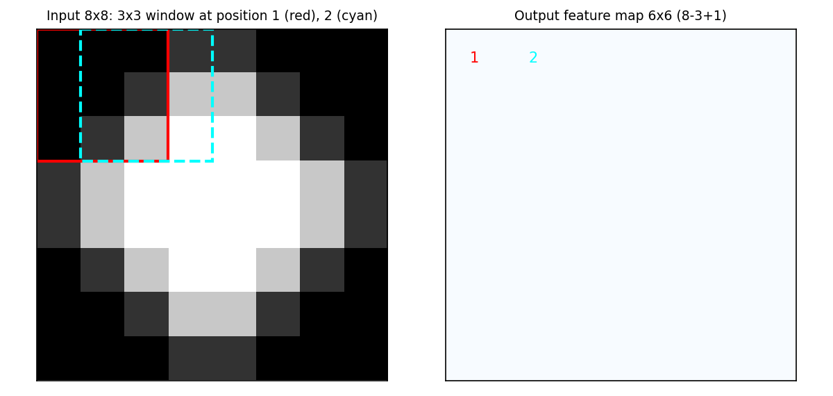
Output sizeSliding a 3×3 filter over an 8×8 image, staying fully inside the image, gives a 6×6 output (), as drawn on the slide. In general an image and filter give . The slides do not discuss padding. (Reconstructed.)
The three filters
| Filter | Kernel | Effect | Use |
|---|---|---|---|
| Edge (vertical) | [[-1,0,1],[-2,0,2],[-1,0,1]] |
Highlights left-to-right brightness jumps | Shapes, contours, outlines |
| Blur (average) | 3×3 of 1/9 | Replaces a pixel with its neighbourhood mean, smooths noise | Pre-processing, soft backgrounds |
| Sharpen | [[0,-1,0],[-1,5,-1],[0,-1,0]] |
Amplifies difference from neighbours | Texture, crisper thumbnails |
Worked: edge filter at position (2,2) of the plateNeighbourhood (rows R1 to R3, cols C1 to C3):
[[0,50,200],[50,200,255],[200,255,255]]
- Row 1:
- Row 2:
- Row 3:
Total = 665: a strong vertical edge (the plate rim). The filter does not "know" about plates; it only finds where brightness changes sharply. High values form a ring along the rim, near zero in the uniform centre and corners.
Worked: blur at position (3,3)Neighbourhood
[[200,255,255],[255,255,255],[255,255,255]]. Average . The centre stays bright because the area is uniformly bright; blur matters most at transitions.
Worked: sharpen at position (2,3)Neighbourhood
[[50,200,200],[200,255,255],[255,255,255]].
- Row 1:
- Row 2:
- Row 3:
Total = 365. Sharpen exaggerates jumps at the rim and leaves uniform areas roughly unchanged.
I recomputed all three filters over the whole plate (valid positions); the values at the three positions above match the slides (665, 249, 365):
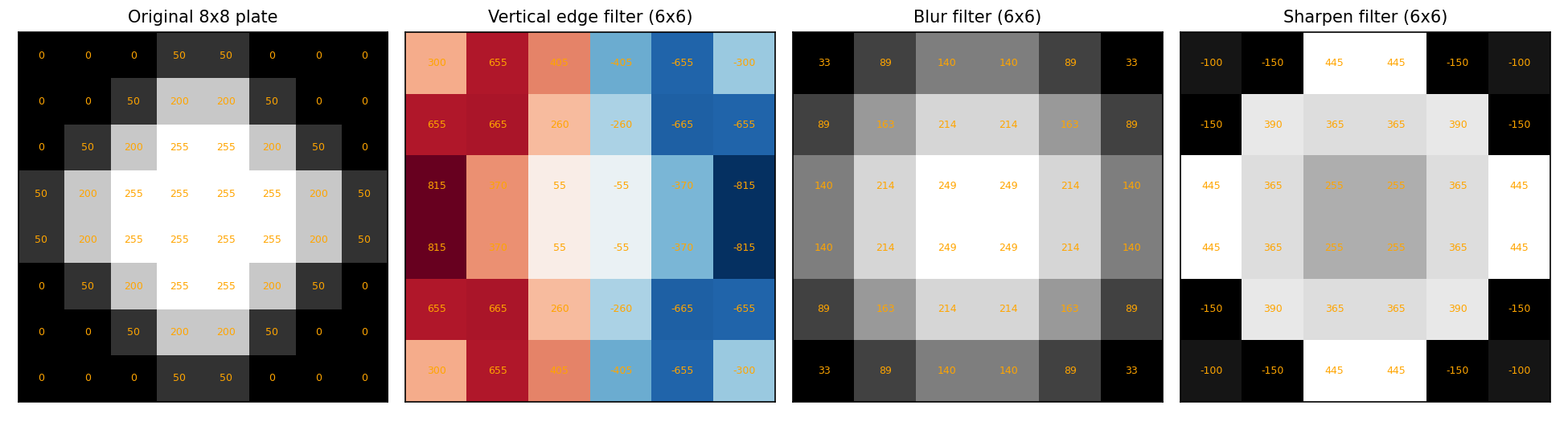
ReconstructedThe figure above is not on the slides; it is my full-grid computation of the three filters on the demo plate (red = positive edge response, dark to light; blue = negative, light to dark). The edge filter responds with opposite signs on the left and right rim, so a "strength" feature should use absolute values.
import numpy as np
from scipy.signal import correlate2d

edge_filter = np.array([[-1, 0, 1],
                        [-2, 0, 2],
                        [-1, 0, 1]])
feature_map = correlate2d(plate, edge_filter, mode="valid")  # slide, multiply, sum
feature_map.shape       # (6, 6)
feature_map[1, 1]       # 665, the slide's worked example
Not from the slides
correlate2d(..., mode="valid")performs exactly the slide's slide-multiply-sum without kernel flipping; the equivalent loop reproduces 665, 249 (1/9 kernel) and 365.
Filter size
| Size | Numbers | Detects | Note |
|---|---|---|---|
| 3×3 | 9 | Fine details (thin edges, small textures) | Most common |
| 5×5 | 25 | Thicker edges, medium textures | |
| 7×7 | 49 | Large-scale patterns (gradients, broad shapes) | More context, more compute, can blur fine details |
Many filters, one rich description
One filter finds one pattern type. Real systems apply dozens or hundreds of filters; the stack of feature maps is a numeric description of the image, just as the DTM describes a review.
| NLP (BoW) | Images (filters) | |
|---|---|---|
| Raw input | Text sentence | Pixel grid |
| Feature extraction | Count each word | Apply each filter |
| Output | Document-term matrix | Stack of feature maps |
| Each feature | Count of one word | Response to one filter |
| Ready for | Classification, clustering | Classification, detection |
CNNs (teaser for Lecture 8)
A CNN (Convolutional Neural Network) is a deep-learning model that learns its own filters from thousands of labelled images instead of using hand-designed ones (edge, blur, sharpen). We hand-designed 3 filters; a CNN is given, say, 100 blank filters and 10,000 labelled photos and works out which patterns matter. Continued in Lecture 8 - Intro to Deep Learning.
Not covered (but exist): word embeddings (Word2Vec, GloVe) that fix the synonym problem; transformers and LLMs; object detection; transfer learning (fine-tuning a pre-trained model).
Hands-on exercises
Exercise 1: NLP for Balagan Café (1,000 reviews, 15 cafés)
- Pipeline: lowercase, remove punctuation, tokenize, remove stopwords, lemmatize.
- DTM shape with an 800-word vocabulary: , very sparse.
- "wait" (200 reviews) mostly co-occurring with "coffee" (350) suggests complaints about coffee wait times, not table waits: investigate barista staffing and equipment.
- High similarity between "wifi" and "outlet" reviews means customers see them as one topic (digital workspace): treat as a single improvement project.
- Limitation: BoW misses sarcasm and negation, e.g. "The coffee was NOT bad" registers
coffeeandbad.Recommendation: prioritise coffee speed, bundle wifi and outlets, and remember the analysis may miss nuanced reviews.
Exercise 2: plated dish vs close-up (4×4 grids)Photo A (plated): border of 20s around a 2×2 centre of 200s. Photo B (close-up): smooth gradient from 180 to 215.
- A looks like a bright plate on a dark surface; B is a gentle texture gradient.
- Edge detection gives higher values on A (jump of 180 between neighbours) than B (differences of 5 to 15).
- Feature idea: compute the mean edge strength of the feature map; high = plated, low = close-up, and feed it to a classifier.
- Blur is least useful: it smooths away the very edges needed.
Exercise 3: Sababa Eats (5,000 reviews, 10,000 photos, 200 restaurants)
- Text: the full pipeline then BoW. DTM ; average each restaurant's review vectors to get a restaurant matrix.
- Images: apply filters to each photo, take summary statistics (mean edge strength, mean brightness, texture score = variance of pixel values), average per restaurant: about 5 to 10 numbers each.
- Combine: concatenate into one wide row: (2,000 text + 10 image columns).
- Recommend: content-based filtering from Lecture 6 (cosine similarity between restaurants) or cluster restaurants (K-Means) and recommend within clusters.
- Challenge: scale mismatch: 2,000 sparse 0/1 text features dominate about 10 dense 0 to 255 image features, so normalise first (StandardScaler, Lecture 5).
Summary
- About 80% of business data is unstructured; models need a numeric matrix, so we must translate.
- Text: lowercase → remove punctuation → tokenize → remove stopwords → stem/lemmatize → Bag-of-Words → document-term matrix (docs × words, counts). Sparse; cosine similarity applies; TF-IDF reweights rare words.
- BoW blind spots: word order, synonyms, context, negation; plus sparsity and high dimensions.
- Images are already numbers: grayscale = 2D (0 to 255), RGB = 3D (H × W × 3). Raw pixels are too many, lack spatial structure and are not shift-robust.
- Convolution = slide, multiply, sum a small filter over the image to produce a feature map. Edge, blur and sharpen are three filters; many filters give a rich feature description.
- A CNN learns its own filters; that is Lecture 8.
- Both pipelines end in the same place: numeric features feeding models from Lectures 3 to 6.
| Lecture | Input | Output | Technique | Challenge |
|---|---|---|---|---|
| 3 Classify | Features + labels | Label | DT, LR, KNN, RF | Overfitting |
| 4 Regress | Features + numbers | Number | Linear, Poly, Ridge, Lasso | Overfitting |
| 5 Cluster | Features only | Clusters | K-Means | Choosing K |
| 6 Recommend | User-item ratings | Predicted ratings | CB, CF, Hybrid | Sparsity |
| 7 NLP & Vision | Raw text / images | Numeric features | BoW, filters | Vocabulary, scale |
Related notes
- Data Science (hub)
- Lecture 6 - Recommendation Systems | Lecture 8 - Intro to Deep Learning
- Lecture 5 - Clustering and Dimensionality Reduction (K-Means, scaling) and Lecture 3 - Classification, KNN, Random Tree (classifiers on a DTM)