
Lecture 6 — Recommendation Systems: How Does Everyone Know What You Want?
- #data-science
- #intro-data-science
- #recommendation-systems
- #content-based-filtering
- #collaborative-filtering
- #cosine-similarity
- #cold-start
- #hybrid-recommender
- #evaluation
- #pandas
- #scikit-learn
Lecture 6 — Recommendation Systems
Part of: Data Science Previous: Lecture 5 - Clustering and Dimensionality Reduction | Next: Lecture 7 - NLP and Image Analysis Key concepts: Recommendation System, User-Item Matrix, Sparsity, Content-Based Filtering, Collaborative Filtering, Cosine Similarity, Cold Start Problem, Hybrid Recommender, Precision at K
The Core Idea
You open a streaming app with 50,000 titles and within 90 seconds you are watching something you love. Recommendation systems are how it knows.
The course arc so far: classify (Lec 3), predict numbers (Lec 4), find groups (Lec 5). Today: predict what an individual will like.
From groups to individualsSegmentation (clustering) says "you belong to the Drama Buffs segment". Personalization says "you specifically would rate THIS show 4.5". Same data skills, finer grain.
Running case study: Seret+A Tel Aviv streaming platform with 200 subscribers, 50 shows (Israeli and international) and a 12% monthly churn rate. Every subscriber sees the same "Trending Now" homepage and the "recommended for you" emails have an open rate below 5%. The CEO's question: can you show each subscriber the shows THEY would actually like? We build the answer three ways (content-based, user-based CF, item-based CF), then combine them.
1. Why Recommend? The Business Case
Paradox of choice. With 1,000 titles, browsing works. With 50,000+, users get decision paralysis, browse for ages, watch nothing and cancel. The fix is to show the right things, not everything.
| Platform | Recommender | Claim on the slides |
|---|---|---|
| Netflix | Personalised homepage | about $1B per year saved in reduced churn (estimate) |
| Spotify | Discover Weekly (30 new songs each Monday) | streamed billions of times |
| Amazon | "Customers who bought X also bought Y" | about 35% of purchases |
| YouTube | Algorithmic feed | about 70% of time on platform |
| Booking.com | "Properties similar to ones you viewed" | n/a |
These figures are quoted from the lecture slides (no sources given), so treat them as illustrative.
Key insightRecommendations are not a feature, they are the core business model. If the algorithm breaks, engagement collapses.
Why "most popular" is not enough
The simplest "recommendation" is the same Top 10 for everyone. A thriller fan and a documentary lover see the same list, so one of them bounces. Personalization gives each user their own list.
The long tail
A long tail (power-law) distribution is one where a few items account for a large share of the total, while a very large number of items each contribute a little. The famous version is the 80/20 rule (Pareto principle): 80% of sales from 20% of products. Other examples: word frequency (Zipf's law), city populations, website traffic.
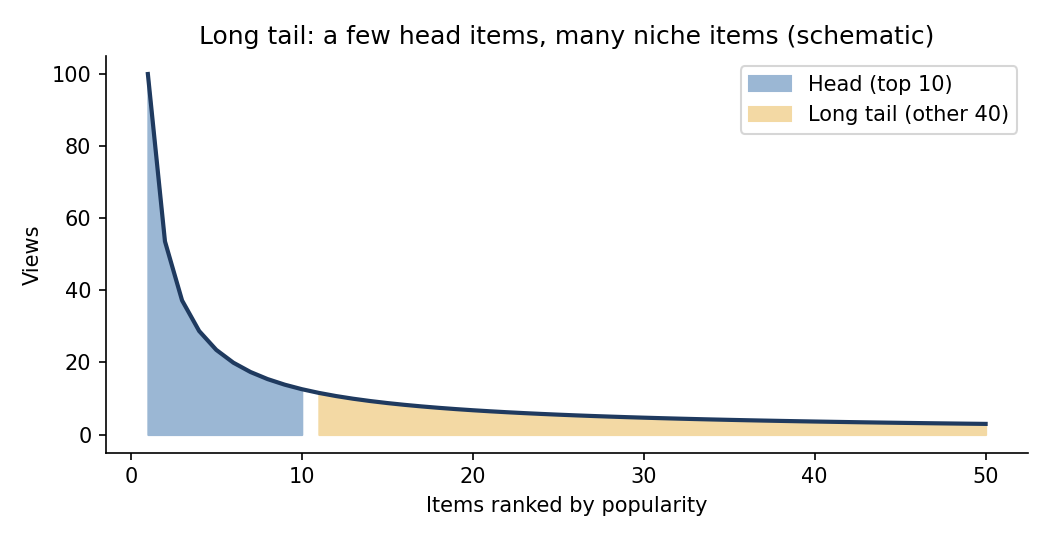
Schematic, not the Seret+ data.
- In a catalogue, the head is a handful of bestsellers; the tail is the many niche items.
- For Seret+ the top 10 shows get 40% of views, but the other 40 shows together get 60%. Without a recommender those 40 shows are invisible; with one, each finds its audience.
- The head is predictable (everyone watches the top 10). The tail is where individual differences live, so that is where personalization adds the most value.
2. What Is a Recommendation System?
DefinitionA recommendation system is an algorithm that predicts how much a user would like an item they have not seen yet, and suggests the items with the highest predicted ratings.
Vocabulary
| Term | Meaning |
|---|---|
| User | A person interacting with the system (subscriber, customer, listener) |
| Item | A thing to recommend (show, product, song, article) |
| Rating | A user's expressed preference (1 to 5 stars, thumbs up/down) |
| User-item matrix | Users as rows, items as columns, ratings as values |
| Sparsity | Percentage of the matrix with no rating (typically 95 to 99%+) |
| Prediction | Filling in a missing cell: what would this user rate this unseen item? |
The user-item matrix: the core data structure
This 8-user by 10-item subset is the demo matrix used for every hand calculation below. ? means "not rated".
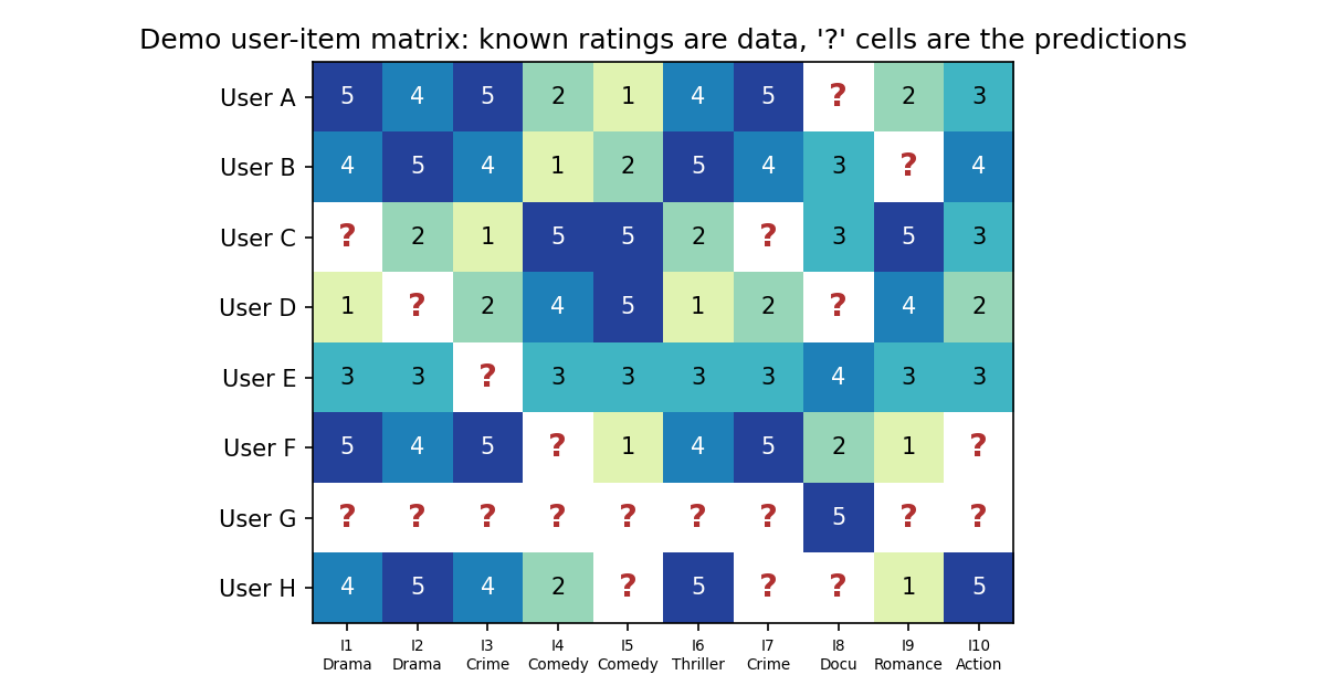
Key insightThis matrix IS the recommendation problem. Known ratings are data; empty cells are predictions to make. Every recommender is, at its core, a method for filling in the blanks.
Reading the demo matrix:
- A, B, F, H: Drama Buffs (dramas and thrillers high, comedies low).
- C, D: Comedy Lovers (the opposite pattern).
- E: Omnivore (rates almost everything about 3).
- G: Cold start: has rated only one item (I8).
- Target prediction for the whole lecture: what would User A rate I8 (a documentary)?
How sparse is sparse?
Netflix has roughly 200 million users and 15,000 titles: about 3 trillion cells. The average user rates about 200 titles, so the matrix is about 99.999% empty. Even small Seret+ is 80% empty.
Sparsity is not a data-quality bugUsers will never rate everything. Sparsity is the nature of the problem, and coping with it is the central challenge.
Explicit vs implicit feedback
| Explicit | Implicit | |
|---|---|---|
| Example | 4.5-star rating | Watched 95% of the show |
| Signal quality | Clear | Noisy (watched but fell asleep?) |
| Availability | Rare, most users do not rate | Abundant, every click is data |
| Seret+ column | rating |
watch_pct |
Mismatch problem: rating is not the same as watching. Someone may rate a show 3 stars but watch 100% (a guilty pleasure), or rate 5 stars but watch only 40% (rating what they think they should like). When the two disagree, implicit is often more honest, but this lecture uses explicit ratings because they are cleaner to evaluate.
What recommenders are NOT
- Not search engines: search needs a query, recommendation is proactive.
- Not just "show the most popular": that is a fallback, not personalization.
- Not magic: with zero data they fail (cold start, section 6).
- Not neutral: they shape what people see and can create filter bubbles.
A good recommender balances relevance (show what the user will like) with discovery (introduce content they would not find alone).
3. Meet the Data: Seret+
Three related tables, joined by two keys. This is the first time in the course we work with multiple related tables.
| Table | Rows | Columns |
|---|---|---|
ratings.csv |
2,000 | user_id, item_id (join keys), rating (1.0 to 5.0, explicit), watch_pct (0 to 100, implicit), timestamp |
items.csv |
50 | item_id, title, genre, sub_genre, language (HE / EN / AR), release_year, avg_episode_min, num_seasons, is_original |
users.csv |
200 | subscriber profiles (4 columns) |
ratings connects users to items: user_id links to users, item_id links to items.
import pandas as pd

ratings = pd.read_csv("seret_ratings.csv")
items = pd.read_csv("seret_items.csv")
users = pd.read_csv("seret_users.csv")

print(ratings.shape)  # (2000, 5)
print(items.shape)    # (50, 9)
print(users.shape)    # (200, 4)
Quick EDA (from the slides)
| Metric | Value |
|---|---|
| Rating mean / std | about 3.4 / about 1.1 |
| Rating min / max | 1.0 / 5.0 |
| Watch % mean / std | about 65 / about 28 |
| Unique users / items | 200 / 50 |
| Avg ratings per user / per item | about 10 / about 40 |
Each user has rated about 10 of 50 shows, only 20%, so predictions must come from very little information.
import matplotlib.pyplot as plt

ratings["rating"].hist(bins=9, color="teal", edgecolor="black")
plt.xlabel("Rating")
plt.title("Distribution of Ratings")
The histogram is left-skewed: most ratings sit at 3 to 4 with a peak at 4.0.
Selection biasUsers mostly rate shows they chose to watch, so they probably expected to like them. Ratings skew positive, and a 3 may really mean "disappointed", not "average".
Ratings per user: most have 5 to 15 (median about 10), a few power users 30+. Ratings per item: popular shows 50+, niche documentaries 15 to 25 (median about 40).
Popularity bias (feedback loop)Popular items have many ratings, so the algorithm knows more about them, so they get recommended more, so they become more popular. Niche content gets trapped in obscurity. Remember: the most-rated item is not necessarily the best. A documentary with 20 ratings averaging 4.8 may beat a drama with 60 ratings averaging 3.5.
Building the user-item matrix
pivot_table converts long format (one row per rating) into matrix format (one row per user, one column per item):
matrix = ratings.pivot_table(
    index="user_id",      # rows = users
    columns="item_id",    # columns = items
    values="rating",      # cell = the rating
)

print(matrix.shape)                # (200, 50)
print(matrix.isna().mean().mean()) # about 0.80 -> 80% of cells are empty
matrix.isna().mean().mean() computes the share of NaN cells per column, then averages across columns, which is the overall sparsity.
4. Content-Based Filtering
DefinitionContent-based filtering recommends items that are similar to items the user has already rated highly, with similarity measured on item features (genre, language, length...).
Analogy: a bookstore employee sees you buying three mysteries and says "here are our other top mysteries". They need no knowledge of other customers.
The 4-step pipeline
- Describe each item with a feature vector.
- Build a user profile by averaging the feature vectors of items the user rated highly.
- Compute similarity between the profile and every unseen item.
- Rank and recommend the most similar unseen items.
Step 1: item feature vectors
Categorical features are One-Hot Encoding-ed (as in Lecture 3 - Classification, KNN, Random Tree); drop_first=True avoids redundant columns.
item_features = pd.get_dummies(
    items[["genre", "language", "is_original"]],
    drop_first=True,   # avoid redundancy (as in Lecture 3)
)
item_features.head()
Result shape (slide excerpt): one row per item, e.g. I1 (Fauda) has Drama=1, Hebrew=1; I4 (comedy) has Comedy=1, Hebrew=1; I8 (documentary) has Docu=1, English=1.
Cosine similarity: how we measure "similar"
DefinitionCosine similarity measures the angle between two vectors, not the distance. It ranges from (opposite) to (identical direction). For non-negative feature vectors it ranges from (nothing in common) to (identical).
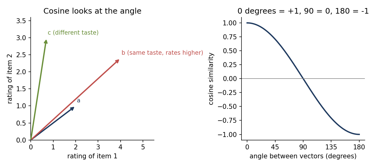
Why not Euclidean distance? (Euclidean Distance, used in K-Means and KNN.) Euclidean measures how far apart two points are; cosine measures whether they point the same way. Two users with the same taste pattern but different rating scales (one rates 4 to 5, the other 2 to 3) are far apart by Euclidean distance but near-identical by cosine. Rating vectors are also sparse and on personal scales, so cosine ignores magnitude and focuses on pattern.
Worked example: I3 vs I7 (both Hebrew crime dramas)Feature columns: Drama, Crime, Hebrew, English, Original, Other.
Drama Crime Hebrew English Original Other I3 1 1 1 0 1 0 I7 1 1 1 0 0 0
- Dot product:
- ,
- (very similar)
Compare I3 vs I4 (crime drama vs comedy): cosine about 0.10 (slide value), very different.
Step 2: build a user profile
DefinitionA user profile is the average feature vector of the items the user rated highly (say 4 or above). It summarises their taste in feature space.
User A rated 4 or higher: I1 (Drama), I2 (Drama), I3 (Crime Drama), I6 (Thriller), I7 (Crime Drama). Averaging those five vectors gives a profile heavy on Drama, Crime, Thriller and Hebrew: "User A loves Hebrew dramas and thrillers".
Steps 3 and 4: score and recommend
Compute cosine between the user's profile and every unseen item, then turn similarity into a predicted rating (a similarity-weighted average of the user's known ratings). For User A:
- I8 (documentary): cosine with A's profile about 0.25 (low)
- I9 (romance): cosine about 0.15 (lower still)
- Predicted A to I8: about 2.8
from sklearn.metrics.pairwise import cosine_similarity

# User A's profile: average features of the liked items
user_profile = item_features.loc[liked_items].mean()

# cosine similarity of the profile to every item (one row of scores)
scores = cosine_similarity([user_profile], item_features)[0]

# Top-5 unseen items
unseen = [i for i in range(50) if i not in rated]
top5 = sorted(unseen, key=lambda i: scores[i], reverse=True)[:5]
liked_items is the list of item indices A rated 4 or above; rated is every item A has rated. sorted(..., key=scores, reverse=True) ranks unseen items from most to least similar.
Strengths and weaknesses
| Strengths | Weaknesses |
|---|---|
| No cold start for items: a new show can be recommended from its features | No serendipity: only more of what you already liked |
| Transparent: "because it's a Hebrew crime drama like your top 5" | Feature engineering needed; coarse genres make all dramas look alike |
| Independent of other users: works with one user | Misses cross-genre gems (comedy-thriller loved by comedy fans) |
| Good for niche items with few ratings | New-user problem remains: no ratings, no profile |
Key insightContent-based plays it safe: accurate but boring (like only suggesting Italian restaurants because you once ate pasta).
Use it when: item features are rich, new items arrive often, explainability matters, or the platform has few users. Avoid it when: features are weak, you want to surprise users, you have plenty of interactions, or diversity is a priority.
5. Collaborative Filtering (CF)
DefinitionCollaborative filtering recommends items from the collective behaviour of all users: if two users agreed in the past, they will likely agree on new items. It uses no item features at all, only rating patterns.
Content-based reads the ingredient list; CF asks someone who ate the dish. CF captures nuance that features cannot: two crime dramas can have identical features while one is beloved and the other mediocre, and only ratings reveal the difference.
5a. User-based CF
Intuition: you move to a new city. Instead of reading restaurant descriptions, find a local who liked the same places you did and ask what else they love.
Step 1: find similar users. Compute cosine similarity between users' rating vectors, using only the items both have rated (the overlap). With zero overlap there is no similarity; the more overlap, the more reliable it is.
Worked example: User A vs User BOverlapping items: I1, I2, I3, I4, I5, I6, I7, I10 (8 items).
I1 I2 I3 I4 I5 I6 I7 I10 A 5 4 5 2 1 4 5 3 B 4 5 4 1 2 5 4 4
- ,
A and B are taste twins. The slide gives cosine(A, C) of about (the "anti-twin"), so CF trusts B and ignores C when recommending to A.
Check on the slide's A vs C numberComputing plain cosine on the raw ratings over the shared items gives A vs C of about +0.66, not (the same plain calculation gives A vs B 0.97, matching the slide). The slide's negative value only makes sense after mean-centering (see below), where I get about . The slide's A vs E value of 0.45 is likewise not reproduced by either method (raw about 0.92, mean-centered about 0.14). Treat the exact neighbour similarities as illustrative; the lesson (B is a twin, C is the opposite) holds.
Step 2: predict from neighbours. Find A's most similar users who have rated I8, then take a similarity-weighted average of their ratings:
Mean-centering subtracts each user's own average rating first. A user who rates everything 4 to 5 and gives a 3 is "disappointed"; one who rates 1 to 3 and gives a 3 is "impressed". Mean-centering turns raw ratings into deviations from each user's baseline.
Worked example: A to I8Neighbours who rated I8: B (sim 0.97, rated 3), E (sim 0.45, rated 4), F (sim 0.95, rated 2).
The slide then says mean-centering adjusts this to a final prediction of about 2.6.
Check on the mean-centred 2.6Using the slide's similarities and the demo matrix, mean-centring A's I8 prediction gives about 2.8 (A's mean about 3.44, neighbour deviations at I8 of about , , ), not 2.6. The slide's 2.6 is not reproduced from the numbers shown; the qualitative conclusion (A is not a documentary fan) is unchanged.
from sklearn.metrics.pairwise import cosine_similarity
import numpy as np

# user-user similarity on the rating matrix
matrix_filled = matrix.fillna(0)   # NaN -> 0
user_sim = cosine_similarity(matrix_filled)

# Predict: weighted average of K nearest neighbours
# (simplified -- production code handles NaN properly)
Filling NaN with 0 treats "not rated" as "rated 0", which is why the slide marks this as simplified.
Choosing K. Too few neighbours means noisy predictions; too many dilutes taste differences (ask 1 friend: strong but maybe wrong opinion; ask 100 strangers: bland average; 5 to 20 close friends is the sweet spot). Typical to depending on size and sparsity.
Connection to Lecture 3This is the same idea as KNN: there, neighbours voted on a label; here, neighbours vote on a rating.
Strengths: finds unexpected gems ("users like you loved this documentary"), needs no item features, captures subtle taste, delivers serendipity.
Problems:
- Sparsity hurts: two users overlapping on only 2 items give an unreliable similarity.
- Scalability: similarity between all user pairs is expensive with millions of users.
- Popularity bias: popular items have more neighbours who rated them.
- Users change: old ratings keep influencing recommendations (asking high-school friends who knew the old you).
Thin overlap means thin evidenceA cosine of 0.95 from 2 shared items is far less trustworthy than 0.85 from 15 to 20 shared items. Some implementations require a minimum overlap before trusting a similarity.
5b. Item-based CF
DefinitionItem-based CF recommends items similar to ones the user already liked, but similarity is measured from rating patterns, not features. Two items are similar if the same users tend to rate them similarly.
Content-based says "both are dramas". Item-based CF says "everyone who liked A also liked B, regardless of genre".
Why item-based often beats user-based
- Stability: items do not change; users' tastes drift.
- Scalability: millions of users but "only" 50,000 items gives a much smaller item-item matrix.
- Precomputation: the item-item matrix can be computed once and reused for all users; user-user must be recomputed as users join.
Step 1: item-item similarity uses the columns of the matrix.
Worked example: I3 vs I7 (users who rated both: A, B, D, F)
- ,
- , identical reception.
Step 2: predict from similar items. Take the items most similar to the target that the user has rated, and average the user's own ratings of them, weighted by item similarity:
Worked example: A to I8Most similar rated items (slide values): I10 (Action, sim 0.35, A rated 3), I9 (Romance, sim 0.20, A rated 2), I4 (Comedy, sim 0.15, A rated 2).
# item-item similarity from the rating matrix
matrix_T = matrix_filled.T            # transpose: items as rows
item_sim = cosine_similarity(matrix_T)  # 50 x 50 item similarity matrix
item_sim_df = pd.DataFrame(
    item_sim,
    index=items["title"],
    columns=items["title"],
)
Amazon's "also bought" IS item-based CF"Customers who bought this also bought..." computes which products are co-purchased, then recommends the most similar items to what is in your cart. For Seret+: "Viewers who enjoyed Fauda also enjoyed Tehran, Shtisel, The Beauty Queen of Jerusalem".
Comparing the three approaches
| Content-based | User-based CF | Item-based CF | |
|---|---|---|---|
| Uses | Item features | User rating patterns | Item rating patterns |
| Similarity between | Items (features) | Users (ratings) | Items (ratings) |
| A to I8 prediction | about 2.8 | about 2.6 | about 2.5 |
| Serendipity | Low (same genre) | High (taste twins) | Moderate |
| New item | Works | Needs ratings | Needs ratings |
| New user | Needs ratings | Needs ratings | Needs ratings |
| Scalability | Fast | Slow () | Medium () |
| Explainability | High | Medium | High |
All three agree: User A will not love this documentary. No single approach wins everywhere.
| Situation | Best approach | Why |
|---|---|---|
| New platform, few users, good metadata | Content-based | CF needs critical mass |
| Mature platform, millions of users | Item-based CF | Scalable, stable, proven |
| Niche platform, tight community | User-based CF | Small user base is manageable |
| Any serious production system | Hybrid | Combines strengths |
6. The Cold Start Problem
DefinitionThe cold start problem is when the system has too little data to make good predictions. Two cases: a new user with zero ratings, or a new item with zero ratings.
Analogy: a new employee on day one (nobody knows their style), or a restaurant that just opened (no reviews).
New user (User G, one rating: I8 = 5)
| Approach | What it can do |
|---|---|
| Content-based | Barely works: a profile from one documentary, so it recommends more documentaries (G may be an omnivore who rated a docu first) |
| User-based CF | No meaningful neighbours (1 overlapping item) |
| Item-based CF | Only items similar to I8: very narrow |
With one rating, all approaches are essentially guessing.
New item (Item 50, only 3 ratings from users 10, 55, 120)
| Approach | What it can do |
|---|---|
| Content-based | Works fine: features exist from day one, ratings not needed |
| User-based CF | Only 3 ratings to learn from |
| Item-based CF | Very few co-ratings, so unreliable |
Key insightContent-based handles new items well; CF struggles because it needs rating history. This is a key reason to keep content-based in the toolkit.
Practical solutions
| Strategy | How it works | When to use |
|---|---|---|
| Popularity fallback | Show the most popular items | Brand-new users (day 1) |
| Onboarding quiz | Ask new users to rate 5 to 10 items | During signup |
| Demographic defaults | Use age, location, language | When profiles exist |
| Content-based first | Recommend by features until ratings accumulate | New items with good metadata |
| Hybrid | Start content-based, blend in CF as data grows | Production best practice |
Seret+ plan: Day 1, "Most Popular in Israel". After 3 ratings, switch to content-based. After 10 ratings, blend in collaborative filtering.
Why it is a business crisis: the churn windowThe first 7 days decide whether a new subscriber stays. The recommender has almost no data then, so an irrelevant homepage drives them away, and they never generate the ratings that would have improved recommendations. It is a chicken-and-egg problem: you need ratings to recommend well, but need good recommendations to get ratings. Every cold-start strategy is a compromise (popularity is generic, quizzes add friction, demographic defaults can stereotype), so combine strategies and graduate to CF as data accumulates.
7. Combining Approaches: Hybrid Recommenders
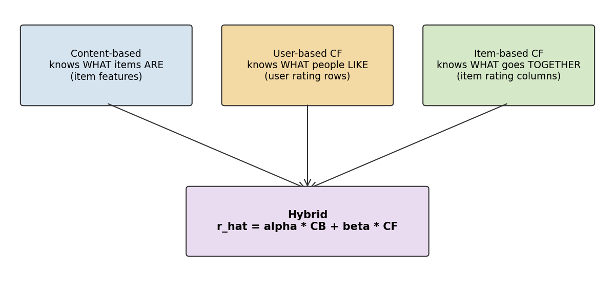
Each approach has blind spots: content-based lacks serendipity, CF fails on cold start, item-CF needs rating density. A hybrid covers each one's weaknesses.
Weighted hybridBlend content-based (CB) with item-based CF (chosen because it scales better):
Worked example: A to I8CB prediction 2.8, item-CF prediction 2.5, with , :
The weights are tunable: for new users (few ratings) raise (trust content-based); for active users raise (trust CF). It is like a second opinion from a specialist.
# Weighted hybrid (illustrative, not from the slides)
alpha, beta = 0.4, 0.6
hybrid_prediction = alpha * content_pred + beta * item_cf_pred
A glimpse beyond: matrix factorization
Matrix factorization decomposes the user-item matrix into two smaller matrices (user-taste and item-taste). Each user and item gets a short vector of latent factors, hidden taste dimensions discovered from rating patterns (e.g. "action lover", "art-house fan"). Think of it as PCA for recommendations: PCA found hidden "super-features" like spending power; matrix factorization finds hidden taste dimensions. These factors are not labelled by hand.
Real-world pipelines
| Stage | What happens |
|---|---|
| 1. Candidate generation | 50,000 items narrowed to about 500 candidates |
| 2. Ranking | Score the 500 with a hybrid model |
| 3. Re-ranking | Business rules: diversity, freshness |
| 4. Presentation | Top 10 to 20 in personalised order |
Key insightNo production system uses one algorithm (Netflix runs dozens in an ensemble with business rules on top). The algorithms are the engine; business rules are the steering wheel.
Strategy by business situation
| Situation | Approach |
|---|---|
| New platform, under 1,000 users, good catalogue data | Start with content-based |
| Growing platform, 1K to 100K users | Add item-based CF as ratings grow |
| Mature platform, 100K+ users | Full hybrid: content + CF + business rules |
| Cold start killing churn | Invest in onboarding + content-based fallback |
| Explainability required (healthcare, finance) | Content-based or item-CF ("because you watched X") |
8. Is It Working? Evaluation
Recommender evaluation is harder than classification (accuracy) or regression (RMSE, R-Squared):
- You cannot test recommendations the user never saw.
- A "correct" prediction is not necessarily useful (predicting 3.5 for everything is technically fine but useless).
- Business success (engagement, retention) does not always match prediction accuracy.
Offline evaluation
Hide some known ratings (the test set, e.g. 20%), build the model on the rest (train, 80%), and measure how well it predicts the hidden ratings. This is the Train Test Split idea applied cell-by-cell to the user-item matrix.
Metric 1: RMSE (prediction accuracy, lower is better)
Metric 2: Precision@K (top-N quality)
"Relevant" usually means rated 4 or above.
Worked example: User A, top 5Recommended top 5: I1, I6, I7, I3, I10. User A actually rated 4 or above on I1, I6, I7, I3 (hits) and 3 on I10 (miss). .
This is the CEO's metric: of the 5 shows on the homepage, how many will the subscriber actually enjoy?
Metric 3: Recall@K (coverage)
Precision asks "how many of my recommendations were good?"; recall asks "how many good items did I miss?" (compare Precision and Recall from classification). Improving one often hurts the other. Precision@K matters more for a homepage; Recall@K matters more for search.
import numpy as np

def rmse(predicted, actual):
    """Root mean squared error between predicted and actual ratings."""
    return np.sqrt(np.mean((np.array(predicted) - np.array(actual)) ** 2))

def precision_at_k(recommended, liked_items, k=5):
    """Share of the top-k recommended items the user actually liked."""
    top_k = recommended[:k]
    hits = sum(1 for item in top_k if item in liked_items)
    return hits / k
(These two helper functions were written for these notes, not copied from the slides.)
Seret+ results (slide values)
| Approach | RMSE | Precision@5 | Notes |
|---|---|---|---|
| Popularity baseline (always predict 3.4) | about 1.20 | about 0.35 | Same for everyone |
| Content-based | about 1.05 | about 0.45 | Safe but repetitive |
| User-based CF | about 0.82 | about 0.55 | Better, some serendipity |
| Item-based CF | about 0.78 | about 0.58 | Stable, scalable |
| Hybrid | about 0.71 | about 0.65 | Best overall |
From baseline to hybrid, RMSE drops by about 41% and Precision@5 nearly doubles. A hybrid RMSE of 0.71 means predictions are off by under one star on average.
Beyond accuracy
- Diversity: are recommendations varied? (5 crime dramas in a row is boring.)
- Novelty: are we showing things the user would not find alone?
- Serendipity: do we surprise them in a good way?
- Filter bubble: are we trapping users in a narrow taste?
The best systems optimise for engagement, not just accuracy: a 0.5% RMSE gain does not matter if users get bored.
Online evaluation: A/B testing
Split users into group A (old system) and group B (new system); after 2 to 4 weeks compare watch time, completion rate, retention and churn. A/B testing is the gold standard: offline metrics guide development but do not always predict real-world success.
| Metric | Measures | Use for |
|---|---|---|
| RMSE | Rating prediction error | During development |
| Precision@K | Top-N relevance | Homepage / "For You" |
| Recall@K | Top-N coverage | Search / discovery |
| A/B test | Real-world engagement | Before deploying any change |
9. In-Class Exercises (with solutions from the slides)
Exercise 1: content-based, a new show
Seret+ adds "Tel Aviv Nights": Hebrew romantic drama, 45-min episodes, 1 season, Seret+ original. One-hot features (Drama, Comedy, Docu, Hebrew, English, Original):
| Show | Drama | Comedy | Docu | Hebrew | English | Original |
|---|---|---|---|---|---|---|
| Fauda (I1) | 1 | 0 | 0 | 1 | 0 | 0 |
| HaShminiya (I4) | 0 | 1 | 0 | 1 | 0 | 0 |
| Planet Earth (I8) | 0 | 0 | 1 | 0 | 1 | 0 |
| Tel Aviv Nights | 1 | 0 | 0 | 1 | 0 | 1 |
A. Cosine of Tel Aviv Nights with each show. B. Most similar? C. A user rated Fauda 5, HaShminiya 3, Planet Earth 2: would CB recommend it? D. What limitation does this show?
SolutionA.
- vs Fauda: dot , norms , cosine
- vs HaShminiya: dot , cosine
- vs Planet Earth: dot , cosine
B. Fauda (0.82): they share Drama and Hebrew. C. The profile leans heavily on Fauda (rated 5), so high predicted interest: CB strongly recommends it. D. CB cannot tell quality within a genre; Tel Aviv Nights might be terrible. CB gets the new show recommended immediately (no cold start) but CF would catch poor ratings.
Exercise 2: user-based CF (podcasts, "Hammer Time")
| Pod A (News) | Pod B (Comedy) | Pod C (Tech) | Pod D (Crime) | Pod E (Food) | |
|---|---|---|---|---|---|
| Dana | 5 | 2 | 4 | 5 | ? |
| Eyal | 4 | 1 | 5 | 4 | 3 |
| Noa | 2 | 5 | 1 | 2 | 5 |
| Omer | 3 | 3 | 3 | 3 | 4 |
A. Cosine between Dana and each other user on Pods A to D. B. Most similar? C. Predict Dana's rating for Pod E using the top 2 neighbours. D. New user Yael has zero ratings: can you use user-based CF?
SolutionA. Dana , .
- Eyal : dot , , cosine
- Noa : dot , , cosine
- Omer : dot , , cosine
B. Eyal (0.97), closely followed by Omer (0.96). C. Eyal (0.97, Pod E = 3) and Omer (0.96, Pod E = 4):
D. No: user-based CF needs ratings to compute similarity. Use a popularity fallback, an onboarding quiz, or demographic defaults; solve cold start first.
Exercise 3: strategy for a startup (Balagan Books)
5,000 customers, 20,000 books, 50,000 ratings (about 10 per customer, about 2.5 per book), rich metadata (genre, author, pages, language, year, publisher) and customer profiles. The homepage shows the same bestseller list to everyone and conversion is dropping.
SolutionA. Sparsity: cells, 50,000 filled, so sparsity (far sparser than Seret+'s 80%).
B. Start with content-based: rich metadata, extreme sparsity (CF will struggle), and new books arrive often.
C. Three-phase rollout:
- Phase 1 (weeks 1 to 4): content-based on genre, author, language. Quick, needs no rating density.
- Phase 2 (months 2 to 3): add item-based CF for customers with 10+ ratings; blend with CB in a weighted hybrid.
- Phase 3 (month 4 onward): matrix factorization or a deep-learning model; A/B test against Phase 2; add diversity and freshness constraints.
D. New releases: content-based gives day-one recommendations from metadata; feature the book in "New Releases" for users with matching genre preferences; fold into CF after 50+ ratings.
E. Metric and test: primary Precision@5 (are homepage recommendations clicked?); secondary average order value and time on site. A/B test 50% personalised homepage vs 50% bestseller list for 4 weeks, measuring click-through rate and conversion.
10. Summary
| Content-based | Collaborative filtering | Hybrid | |
|---|---|---|---|
| Input | Item features | Rating matrix | Both |
| Similarity | Item feature cosine | User or item rating cosine | Weighted score |
| Idea | What items are | What people do | Both |
The Seret+ answer: a hybrid reaches RMSE 0.71 and Precision@5 0.65 (nearly 2 of 3 homepage picks are hits); User A (drama fan) gets Hebrew crime dramas and thrillers, User C (comedy fan) gets comedies and romances, and cold start is handled by Popular, then content-based after 3 ratings, then the full hybrid after 10.
The course journey so far
| Classification (Lec 3) | Regression (Lec 4) | Clustering (Lec 5) | Recommendations (Lec 6) | |
|---|---|---|---|---|
| Input | Features + labels | Features + numbers | Features only | User-item ratings |
| Output | Predicted label | Predicted number | Cluster assignment | Predicted ratings |
| Models | DT, LR, KNN, RF | Linear, Polynomial, Ridge | K-Means | CB, user CF, item CF, hybrid |
| Metrics | Accuracy, F1 | MAE, RMSE, R-squared | Silhouette | RMSE, Precision@K |
| Challenge | Overfitting | Overfitting | Choosing K | Sparsity, cold start |
Coming nextLecture 7: text and images (reviews, social posts, support tickets, photographs). Recitation 6 practises the full ratings-to-personalised-top-5 pipeline.
Key Terms
| Term | Definition |
|---|---|
| Recommendation System | Algorithm that predicts user preferences and suggests relevant items |
| Content-Based Filtering | Recommends items similar to what the user liked, based on item features |
| Collaborative Filtering | Recommends based on the rating patterns of similar users or items |
| User-Item Matrix | Table with users as rows, items as columns, ratings as values |
| Sparsity | Percentage of the matrix with no ratings (typically 80 to 99.99%) |
| Cosine Similarity | Directional similarity between vectors ( to ) |
| User Profile | Average feature vector of the items a user rated highly |
| User-Based CF | Finds similar users and uses their ratings to predict |
| Item-Based CF | Finds similar items and uses the user's own ratings of them to predict |
| Cold Start Problem | Inability to recommend when a new user or item has too little data |
| Hybrid Recommender | Combines several approaches for better results |
| Matrix Factorization | Decomposes the user-item matrix into latent-factor matrices |
| Precision@K | Fraction of the top-K recommendations that are relevant |
| Recall@K | Fraction of all relevant items captured in the top K |
| Explicit Feedback | Direct user ratings (stars, thumbs) |
| Implicit Feedback | Preferences inferred from behaviour (watch time, clicks) |
| Filter Bubble | Recommendations narrowing exposure to familiar content only |
| Long Tail | Large number of niche items with individually low popularity |