
Lecture 8 — Introduction to Deep Learning: How Machines Learn to Think
- #data-science
- #intro-data-science
- #deep-learning
- #neural-networks
- #perceptron
- #mlp
- #activation-functions
- #gradient-descent
- #overfitting
Lecture 8 — Introduction to Deep Learning
Part of: Data Science Previous: Lecture 7 - NLP and Image Analysis | Next: none Key concepts: Deep Learning, Perceptron, Activation Function, ReLU, Sigmoid Function, Multi-Layer Perceptron, Forward Pass, Loss Function, Gradient Descent, Learning Rate, Epoch, Overfitting
The Core Idea
In Lectures 2 to 7 you designed the features and the preprocessing. Deep learning lets the model design its own features: you supply raw inputs and an architecture, and training discovers useful combinations of inputs.
| Lectures 2 to 6 | Lecture 7 | Lecture 8 | |
|---|---|---|---|
| Who designs features? | You | You (preprocessing: tokens, filters) | The model |
| Human effort | High | Medium | Low |
| Machine effort | Low | Medium | High |
In plain EnglishLectures 2 to 7: you were a chef choosing ingredients and the recipe. Deep learning is a chef who invents the recipe and discovers ingredients you didn't know existed.
Running case study: DerechA Tel Aviv ride-hailing startup with 2,000 drivers across 10 neighbourhoods. The VP Operations must predict ride demand one hour ahead: too few drivers and customers churn, too many and drivers idle (₪80 per hour wasted). Dataset: 3,000 historical records, 7 input features + 1 target.
Column Type Meaning hourint Hour of pickup request (0 to 23) day_of_weekcat Sun to Sat neighborhoodcat 10 TLV neighbourhoods is_rainingbool Weather is_holidaybool Israeli holiday / special day nearby_eventsint Events ending within 1 km in the next hour historical_avgfloat Average rides per hour for this area demand_levelcat Target: Low / Medium / High / Surge
1. What Can't Our Models See? (the interaction problem)
Derech's best attempts so far (all from Lecture 3 - Classification, KNN, Random Tree):
| Model | Accuracy | Limitation |
|---|---|---|
| Logistic Regression | 61% | Linear: effects only add up |
| Decision Tree | 68% | Splits on one feature at a time, misses complex combinations |
| Random Forest | 72% | Better, but still limited to the features you defined |
The interaction problemRain + rush hour is not "rain effect" plus "rush-hour effect". Their combination (plus a concert) creates Surge demand. Linear models add effects; trees split on one feature at a time. Neither captures the multiplication of effects naturally.
| Hour | Rain | Events | True demand | Linear prediction |
|---|---|---|---|---|
| Evening | Yes | 0 | High | Medium (wrong) |
| Evening | Yes | 1 concert | Surge | High (wrong) |
| Morning | Yes | 0 | Medium | Medium (right) |
The linear model gets the morning right but misses the evening surge, because it can't learn that rain x evening x events is qualitatively different from rain + evening + events.
Why not just add polynomial features?
Lecture 4 - Regression gave us polynomial features, but they mean manually guessing which combinations matter. With 7 inputs there are two-way, three-way and four-way interactions: over 90 new columns, most of them noise, and you are still guessing.
The ceiling of hand-designed featuresDT, LR, RF, bag-of-words (Lecture 7 - NLP and Image Analysis) and image filters all sit below a ceiling: they use features you designed. A neural network sits above it, because it learns its own features. Analogy: a founder who does everything hits a ceiling; hiring specialists who discover opportunities the founder never saw is what hidden layers do.
What is deep learning?
Deep LearningA subfield of ML where models with multiple processing layers (hence "deep") automatically learn representations of data at increasing levels of abstraction. The model discovers features during training instead of the human designing them.
Where it shows up: voice assistants, image recognition (Face ID), language models, recommendation engines, fraud detection, autonomous vehicles, medical imaging.
The landscape: Artificial Intelligence ⊃ Machine Learning (Lectures 1 to 7) ⊃ Deep Learning ⊃ {MLP (today), CNN (images), RNN (sequences), Transformers (ChatGPT)}. The MLP is the simplest foundation; the others build on the same principles.
The promiseAn MLP reaches 83% accuracy on Derech's data versus 72% for the best earlier model, because it learns the feature interactions trees and linear models miss. That is 840 wrong predictions per day falling to 510 (out of 3,000), about 330 more correct driver placements. For simplicity the lecture frames it as binary (High demand vs Not High) with a single output neuron.
Reconstructed from the slidesThe 840 and 510 figures follow from the error rates 28% and 17% of 3,000 records; the slide states the counts and the 330 saving directly.
2. Meet the Perceptron
A perceptron (artificial neuron) is the basic unit: it takes numeric inputs , multiplies each by a weight (its importance), adds a bias , then applies an activation function to produce one output.
In plain EnglishA neuron is a hiring manager reviewing a candidate: inputs arrive (GPA, experience, interview score), each has a different importance (weight), the manager adds them up and decides hire or pass.
Step 1: weighted sum
Derech Scenario A (rainy evening): inputs (hour), (rain), (events); weights ; bias .
Hour contributes 0.4, rain 0.8, events 0: a weighted vote (the bias shifts the decision boundary). But is 1.1 "high demand"? We need one more step.
Step 2: activation function
Two reasons we need one:
- The raw sum is unbounded (it could be -50, 1.1 or 1000); we want a useful range.
- Stacking linear layers is pointless. Without activations, multiple linear layers collapse into one linear layer (matrix multiplication is associative). Activations add non-linearity, which is what makes deep networks powerful.
Why not skip activation?Without activation functions a 100-layer network is mathematically identical to a 1-layer network. They are essential, not optional. (Analogy: a thermostat turns any raw temperature into ON or OFF.)
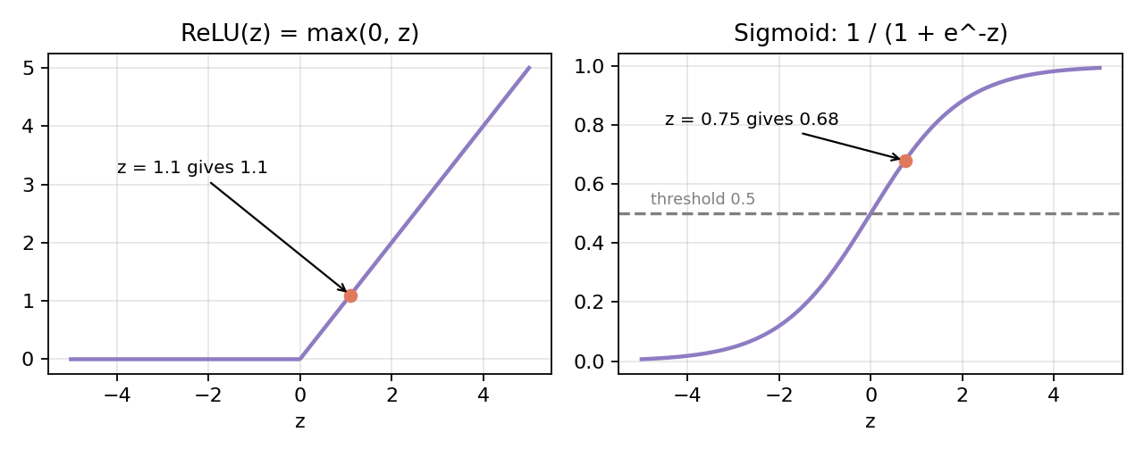
ReLU (Rectified Linear Unit): pass positives, block negatives.
Examples: , , . Dead simple and trains fast (a bouncer: positive signals in, negative turned away).
Sigmoid (Sigmoid Function): squashes any number into , readable as a probability.
Key values: (coin flip), (high confidence), (low confidence), (Scenario A below). It is the same function used inside Logistic Regression.
The standard recipeReLU for hidden layers (fast, simple). Sigmoid for the output layer when you need a probability.
The complete perceptron
For Scenario A with ReLU: . A perceptron = weighted sum + activation function. Every neuron in every network follows this pattern.
What can one perceptron do?
It learns a linear decision boundary, one straight line separating two classes, exactly what Logistic Regression does. It can learn "more rain, more demand" but not "rain matters more in the evening than in the morning" (a non-linear interaction), e.g. classes arranged so no single line separates them.
From one to manyOne expert gives one opinion. A panel of experts, each specialised in a different aspect, gives a much richer assessment. A neural network is that panel; each neuron is a specialist.
3. The Multi-Layer Perceptron (MLP)
A layer is a group of perceptrons that all receive the same inputs and compute in parallel, each with its own weights, so each learns a different pattern. Each neuron in a layer is a feature detector: 2 neurons detect 2 patterns, 100 neurons detect 100, automatically.
The three types of layers
| Layer | Role | Derech |
|---|---|---|
| Input layer | Not really neurons, just the raw features passed in | [hour, is_raining, nearby_events]: 3 nodes |
| Hidden layer(s) | Where the learning happens; "hidden" because you never directly see their outputs | 2 neurons, ReLU |
| Output layer | Produces the prediction | 1 neuron, sigmoid: P(High demand) |
The lecture's MLP (Multi-Layer Perceptron) is a network of fully connected layers like this one.
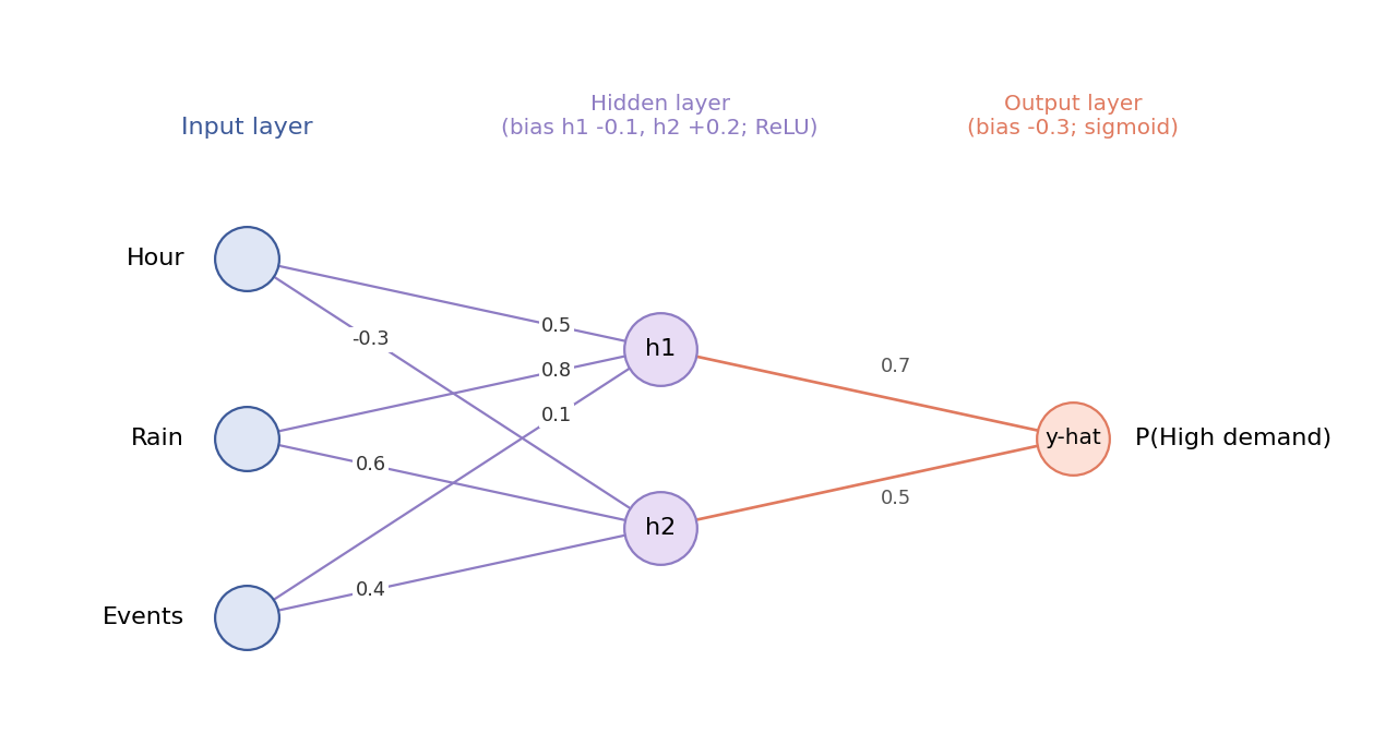
In plain EnglishInput layer = the facts. Hidden layer = the analysis team finding patterns. Output layer = the final recommendation to the CEO.
Why hidden layers matterDerech has
hourandis_rainingas separate columns, but no column for "rainy evening". A hidden neuron can learn to fire strongly when hour is high AND it's raining, effectively creating a "rainy evening" feature no human designed. Hidden neurons create new, abstract features by combining raw inputs.
The forward pass
The forward pass feeds an input through the network left to right, layer by layer: inputs → weighted sums → activation → next layer's inputs (an assembly line: raw materials in, prediction out).
Network parameters used in the lecture (3 inputs, 2 hidden, 1 output):
| Weights | Bias | |
|---|---|---|
| Hidden | hour 0.5, rain 0.8, events 0.1 | -0.1 |
| Hidden | hour -0.3, rain 0.6, events 0.4 | +0.2 |
| Output | from 0.7, from 0.5 | -0.3 |
Scenario A (rainy evening, inputs [0.8, 1.0, 0.0])
Hidden layer:
Output layer:
Scenario B (sunny morning, inputs [0.4, 0.0, 0.0])
| Scenario A (rainy evening) | Scenario B (sunny morning) | |
|---|---|---|
| Inputs | [0.8, 1.0, 0.0] | [0.4, 0.0, 0.0] |
| 1.1 | 0.1 | |
| 0.56 | 0.08 | |
| Output | 0.68, High | 0.45, Not High |
The same forward pass in NumPy (matrix form: one row of hidden_weights per hidden neuron):
import numpy as np

relu = lambda z: np.maximum(0, z)            # keep positives, zero out negatives
sigmoid = lambda z: 1 / (1 + np.exp(-z))     # squash to (0, 1)

hidden_weights = np.array([[0.5, 0.8, 0.1],    # h1: hour, rain, events
                           [-0.3, 0.6, 0.4]])  # h2
hidden_bias = np.array([-0.1, 0.2])
output_weights = np.array([0.7, 0.5])
output_bias = -0.3

def forward_pass(inputs):
    hidden = relu(hidden_weights @ np.array(inputs) + hidden_bias)  # weighted sums, then ReLU
    return hidden, sigmoid(output_weights @ hidden + output_bias)   # output neuron

print(forward_pass([0.8, 1.0, 0.0]))   # h = [1.1, 0.56], probability about 0.68
What did the hidden neurons "learn"?
- (weights 0.5, 0.8, 0.1): a bad-weather + late-hour detector; fires strongly on a rainy evening.
- (weights -0.3, 0.6, 0.4): a daytime rain or events detector: high hour reduces it, rain and events increase it.
Each is an analyst with their own theory; the output layer decides how much to trust each.
Don't over-interpretIn real networks with hundreds of neurons, most hidden features are abstract combinations that don't map to human concepts. They don't need to be interpretable, only useful for prediction.
Width vs depth
- Width = number of neurons in one layer: more patterns detected at the same level of abstraction (more analysts in one department).
- Depth = number of hidden layers: higher-level abstractions built on lower ones (analysts → team leads → directors → VP). The "deep" in deep learning is depth; deeper networks learn more abstract patterns but need more data and training time.
How deep is deep?
| Network | Year | Layers | Parameters | What it does |
|---|---|---|---|---|
| Our demo MLP | Today | 1 hidden | 11 | Predict ride demand |
| AlexNet | 2012 | 8 | 60M | Classify images |
| GPT-3 | 2020 | 96 | 175B | Generate text |
| GPT-4 | 2023 | about 120+ | about 1T+ (rumoured) | General reasoning |
Reconstructed from the slidesThe 11 parameters of the demo MLP check out: hidden layer 2 x (3 weights + 1 bias) = 8, output layer 2 weights + 1 bias = 3.
Bigger isn't always betterFor most business problems a 2-layer MLP with a few hundred neurons is plenty. An oversized model wastes compute and invites Overfitting.
4. How Does It Get Smarter? (training)
Starting pointAll weights start as random numbers. The network knows nothing about rain or rush hour. Like a new employee, it starts with random guesses and improves through feedback. With random weights it might predict 0.52 for Scenario A (true answer: High), barely above the threshold and wrong in spirit.
Step 1: measure the error
A loss function (cost / error function) measures how wrong a prediction is; training aims to make it as small as possible.
- Classification (Derech): compare predicted probability (0.52) with the true label (1.0 for High); the further apart, the higher the loss.
- Regression (Lecture 4 - Regression): squared difference between predicted and true number (familiar from RMSE).
(The lecture gives intuition only, with no loss formulas.)
Step 2: adjust the weights with gradient descent
Gradient descent = walk downhill on the loss surface:
- Start somewhere random (random initial weights give some loss).
- Check the slope: which direction is downhill?
- Take a small step downhill (adjust weights to reduce the loss).
- Repeat until you reach the bottom (minimum).
The learning rate sets the step size.
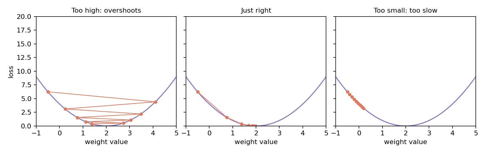
Learning rateToo large: you overshoot and bounce around. Too small: you crawl and waste time. Just right: steady convergence to the minimum. (Figure: a schematic of the slide's three panels on a toy quadratic loss; the step sizes are illustrative.)
Step 3: repeat, the training loop
- Epoch = one complete pass through the entire training set (for Derech: all 3,000 records seen once).
- Training loop: forward pass → compute loss → adjust weights (gradient descent) → next epoch. Typical training is 10 to 100 epochs.
- Slide example: Epoch 1 loss 0.45, Epoch 10 loss 0.12, Epoch 50 loss 0.03.
In plain EnglishTraining is exam prep with practice tests: each test (epoch) you check answers (loss), correct mistakes (adjust weights), and try again.
Overfitting
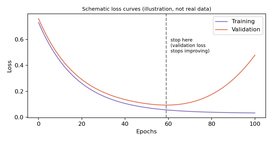
The training loss keeps falling, but the validation loss eventually turns upward: the network has started memorising the training data instead of learning real patterns. The slide splits the curve into fast improvement, refining details and diminishing returns, and says to stop when validation loss stops improving. This is the same overfitting idea as Lectures 3 and 4 (Bias-Variance Tradeoff), amplified because networks have so many weights.
How does each weight get adjusted? (backpropagation, conceptually)
The error at the output is traced backward through the network; each weight is adjusted in proportion to how much it contributed to the error (big contributors move a lot, small ones a little). The math handles this credit assignment automatically.
The relay-team analogyThe team lost; was the anchor slow, or was the baton handoff bad? You trace backward: the final time depends on the anchor, who depends on the third runner, and so on. Each runner gets feedback proportional to their contribution to the loss.
TerminologyThe slides call this step "Backward / trace error back" and never name it. The standard name is backpropagation; no formulas are given.
The full picture
| Step | What happens |
|---|---|
| 1. Initialise | Random weights |
| 2. Forward pass | Data to prediction |
| 3. Loss | How wrong? |
| 4. Backward | Trace error back |
| 5. Update | Adjust weights, then repeat; stop when validation loss stops improving |
| Before | After | |
|---|---|---|
| Weights | Random | Optimised |
| Loss | about 0.7 | about 0.03 |
| Accuracy | about 50% | about 83% |
In practice a library runs this whole loop for you. A Keras-style MLP matching the demo architecture:
from tensorflow import keras

model = keras.Sequential([
    keras.layers.Input(shape=(3,)),                # hour, is_raining, nearby_events
    keras.layers.Dense(2, activation="relu"),      # hidden layer: 2 feature detectors
    keras.layers.Dense(1, activation="sigmoid"),   # output: P(High demand)
])
model.compile(optimizer="sgd", loss="binary_crossentropy", metrics=["accuracy"])
# validation_split holds out data so we can watch for overfitting; 50 epochs is a typical range
model.fit(training_features, training_labels, epochs=50, validation_split=0.2)
Reconstructed, not from the slidesThe Keras snippet above is added to connect the concepts to code. The course addendum says later notebooks use Keras/PyTorch; the Lecture 8 deck itself contains no code.
training_featuresandtraining_labelsare placeholders for Derech's prepared data.
5. Quick Check: trace a forward pass
Scenario C: 2 PM (hour normalised ), not raining (), 2 nearby events (normalised ). Using the same weights:
Prediction: 0.51 > 0.5, borderline High demand, just barely over the threshold.
The business rule51% is barely a "yes". Would the VP deploy extra drivers on 51% confidence? You might raise the threshold (e.g. to 70%) to avoid over-deploying. The sigmoid gives a probability, not just a yes/no, and that tells you how much to trust the prediction: this is where business judgement meets model output.
6. Summary: when to use deep learning
Decision framework
| Factor | Traditional ML (Lectures 3 to 6) | Deep learning (MLP+) |
|---|---|---|
| Data size | Small to medium (100s to 1,000s) | Large (10,000s+) |
| Features | Well understood, hand-designed | Complex interactions, raw data |
| Interpretability | Important (need to explain why) | Less important (need accuracy) |
| Compute | A laptop is fine | May need a GPU for large networks |
| Baseline | Start here always | Add if the baseline isn't good enough |
| Example | Derech with 3K rows | Derech with 300K rows, raw sensor data |
Strengths and weaknesses
| Strengths | Weaknesses |
|---|---|
| Automatic feature learning: finds patterns humans miss | Data hungry: needs lots of labelled data |
| Excels at complex, non-linear interactions | Black box: hard to explain why |
| Scales with data: improves as data grows | Overfitting risk: can memorise training data |
| Universal: same architecture handles tabular, text, image, audio | Compute cost: large networks are expensive to train |
| Overkill for simple problems |
The business questionNot "is deep learning cool?" but "does the accuracy gain justify the extra complexity, cost and loss of interpretability?" Often no; sometimes absolutely yes.
The deep learning checklist
- Have you tried simpler models first? (a baseline is mandatory)
- Enough data? (MLP: 1,000+ rows; CNNs: 10,000+ images)
- Complex feature interactions that simpler models miss?
- Can you tolerate a black-box model? (regulators may say no)
- Do you have the compute? (small MLPs: a laptop is fine)
- Are you monitoring overfitting? (always track validation loss)
If you tick 4 or more, deep learning may be worth trying; otherwise stick with Lectures 3 to 6.
Connecting the full course
| Classification (L3) | Regression (L4) | Clustering (L5) | RecSys (L6) | NLP / Vision (L7) | Deep learning (L8) | |
|---|---|---|---|---|---|---|
| Input | Features + labels | Features + numbers | Features only | User-item ratings | Raw text / images | Any of the above |
| Output | Predicted label | Predicted number | Cluster assignment | Predicted ratings | Numeric features | Predicted anything |
| Key idea | Split on features | Fit a line/curve | Group by similarity | Find similar users/items | Convert to numbers | Learn features automatically |
| Human designs | Features | Features | Features + K | Similarity metric | Preprocessing pipeline | Architecture only |
| Model learns | Decision boundaries | Coefficients | Cluster centres | Weights | (N/A, rule-based) | Features and mapping |
The full journey: Lec 1 What is DS? → Lec 2 Explore → Lec 3 Classify → Lec 4 Predict → Lec 5 Segment → Lec 6 Personalise → Lec 7 Understand → Lec 8 Learn: from data literacy to machine intelligence.
Glossary (from the slides)
| Term | Definition |
|---|---|
| Deep Learning | ML with multiple processing layers that learn features automatically |
| Neuron / Perceptron | Basic unit: weighted sum + activation function |
| Weight | Number controlling how much an input matters |
| Bias | Constant added before the activation (shifts the decision boundary) |
| Activation Function | Non-linear function applied after the weighted sum |
| ReLU | Pass positives, block negatives: |
| Sigmoid | Squashes any number into , a probability |
| Layer | Group of neurons computing in parallel |
| Input / Hidden / Output Layer | Raw features in / middle layers learning abstract features / final prediction |
| MLP | Multi-Layer Perceptron: fully connected layers |
| Forward Pass | Data flowing input → hidden → output |
| Loss Function | Measures how wrong a prediction is |
| Gradient Descent | Adjust weights in the direction that reduces loss |
| Learning Rate | Step size for weight adjustments |
| Epoch | One complete pass through all training data |
| Overfitting | Memorising training data instead of learning real patterns |
Final project briefing
The deck ends with a "Final Project Briefing" section (slides 79 to 81). It contains only a section title, a comic-style image (The Plan / Team Formation / Launch Day) and "Good Luck with Your Projects! See You Next Week!". No project requirements are in the slides; see the course hub for the brief.
Source quirkThe PDF has 81 pages but its footer counts "/ 73" (the title and some section-divider slides are not numbered), so slide numbers printed on the slides differ from PDF page numbers.