
2023 Moed B — Time Preferences & Discounting
Dataset: panel.data — 178 subjects × 15 rounds = 2,670 obs; lab-in-field time-preference experiment, rural Vietnam (2005)
- #econometrics
- #past-paper
- #exam-prep
- #panel-data
- #fixed-effects
- #clustered-standard-errors
- #omitted-variable-bias
- #serial-correlation
- #causal-diagram
- #endogeneity
- #instrumental-variables
- #two-stage-least-squares
- #linear-probability-model
- #difference-in-differences
2023 Moed B — Time Preferences & Discounting
Part of: Econometrics Final Exam 2023 — Moed B — Applied Econometrics, Dr. Aluma Dembo Key concepts: Hypothesis Testing, Omitted Variable Bias, Serial Correlation, Fixed Effects, Individual Fixed Effect, Within Estimator, Clustered Standard Errors, Causal Diagram, Endogeneity, Instrumental Variables, Two Stage Least Squares, First Stage, Second Stage, Instrument Validity, Instrument Relevance, Weak Instruments, Overidentifying Restrictions Test, Wu-Hausman Test, Linear Probability Model, Robust Standard Errors, Difference-in-Differences, Parallel Trends Assumption Builds on: Lec_04-Instrumental Variables, Lec_08-Fixed Effects in Panel Data, Lec_02-Linear Probability Model (LPM), Lec_10-Difference-in-Differences
The Setup (read this first)
A lab-in-field experiment measures time preferences of 178 subjects across 9 rural Vietnamese villages (2005). In each of 15 rounds a subject chooses between Plan A (a larger payment after a delay) and Plan B (a smaller payment today). Each round fixes a A.payment (30k–300k VND) and a A.delay (3–90 days); within the round, five questions vary how much of Plan A is offered today (⅙ → ⅚).
The dataset panel.data is a panel: 178 subjects × 15 rounds = 2,670 obs. The three outcome variables encode the same choice at different resolutions:
| Variable | Type | Meaning |
|---|---|---|
choice |
continuous (0 → ⅚) | fraction of the future payment the subject will forgo to be paid today. Higher = more impatient. |
today.always |
binary | =1 if subject took Plan B (today) on all five questions that round |
delay.always |
binary | =1 if subject took Plan A (delay) on all five questions that round |
The single most important observationWhich outcome a question uses tells you the model.
choiceis continuous → ordinary OLS (Parts A & B).today.alwaysis binary → every regression on it is a Linear Probability Model with heteroskedasticity-robust SEs (Parts C & the DiD in Q4). Spot the outcome type first and you instantly know how to read every coefficient.
The second unlocking idea — what's randomised vs what's observed
A.delayandA.paymentare set by the researcher each round, so they are exogenous — clean regressors. Butincomeis a survey covariate from 2002, not randomised, so it is endogenous (Part B → needs IV). And because it's a panel, the round index and each subject's fixed traits lurk in the error → OVB / fixed effects (Part A). The whole paper is a tour of why the error term is contaminated and the matching fix.
Part A — Does a higher time delay cause higher choice? [Q1, 25 pts]
Outcome
choiceis continuous → OLS. RQ (A): does a longer delay make people prefer money today?
Q1a — Baseline model & null hypothesis [5 pts]
AnswerTo answer RQ (A) we test If a longer delay makes people more impatient we expect ; rejecting answers the question.
Two easy marks people dropInclude the random error and use the subscripts (it's panel data). The official grader docks a point for either omission.
Q1b — Order effects [10 pts]
The worry: in multi-round experiments the round order itself (fatigue, learning) can shift behaviour — "order effects". Note that is not in the baseline model.
AnswerIn the baseline model is hiding in the random error . Round is correlated with the regressors (each round has its own
A.delay/A.payment) and, under order effects, it directly affectschoice. A variable that sits in the error while correlating with a regressor is the definition of an omitted variable — so is biased. The same omitted also makes the errors serially correlated across a subject's rounds.Fix — put in the model: Controlling for removes both problems at once. With the omitted variable now included the errors are no longer serially correlated, so ordinary OLS standard errors are fine — no special correction needed.
graph LR
    round["Round_t (order / fatigue)"] --> delay["A.delay, A.payment"]
    round --> choice["choice"]
    delay --> choice
    class round,delay,choice internal-link;
The backdoor A.delay ← Round → choice is exactly the OVB path; adding blocks it. See OVB, Serial Correlation.
Q1c — Controlling for subject differences with heteroskedastic-by-subject errors [10 pts]
The ask: (i) improve fit by controlling for differences between subjects, and (ii) allow the error variance to differ by subject.
AnswerAdd individual fixed effects (a dummy per subject) to absorb time-invariant differences between people, and cluster the standard errors at the subject level to allow each subject's errors their own variance/correlation.
# Option 1 — explicit dummies, then cluster the SEs by subject
fe1 = feols(choice ~ A.delay + A.payment + factor(id), data = panel.data)
summary(fe1, cluster = ~ id)

# Option 2 — within-estimation; clusters SEs at the FE level automatically
fe2 = feols(choice ~ A.delay + A.payment | id, data = panel.data)
summary(fe2)
Why this is the right toolDifferences between subjects are a per-person intercept . The within estimator (
| id) demeans each subject, so drops out and is identified from within-subject variation only — andfeolsthen clusters byidfor free. Clustering is what "lets the error variance differ by subject": it permits arbitrary within-subject variance and correlation.
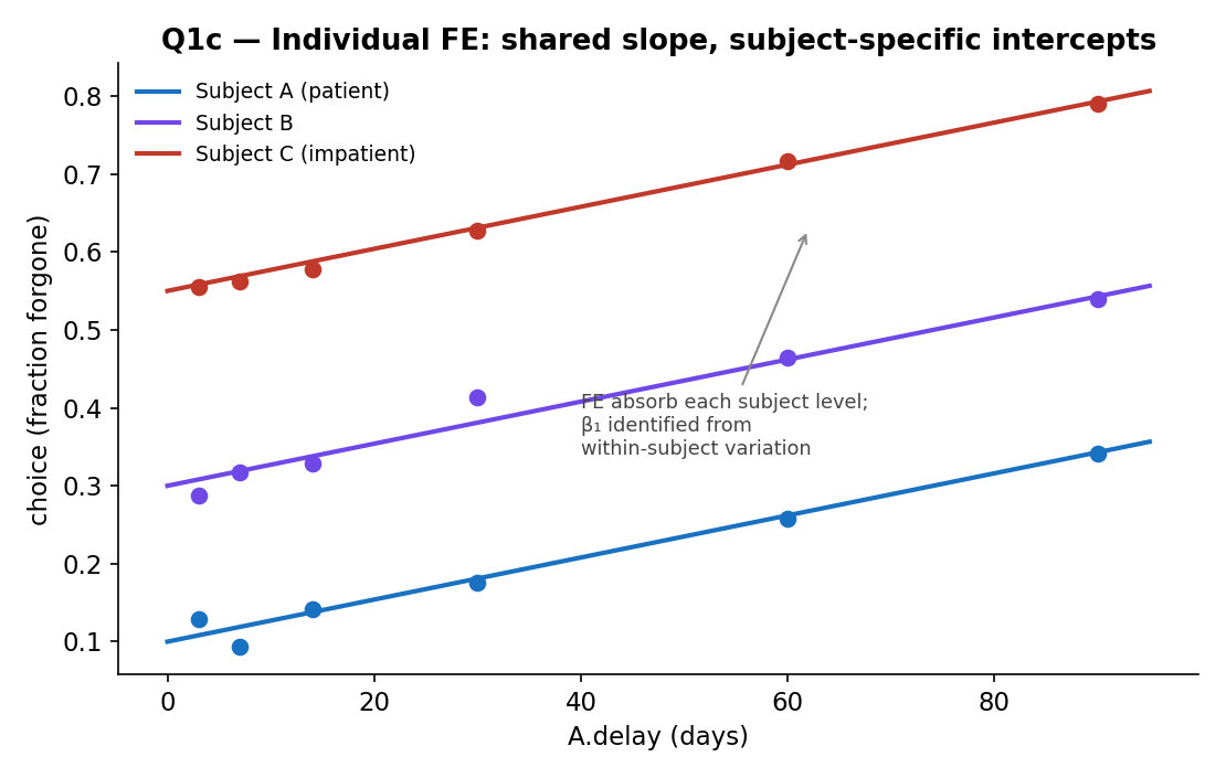
Reading the figure. Each colour is a subject. Fixed effects let every subject keep their own intercept (patient vs impatient baseline) while sharing the same slope — the line's tilt, estimated from how each person moves with A.delay, is the causal object we want.
Own intercept — not own slopeA common slip: thinking FE gives each subject their own intercept and their own gradient. It only shifts intercepts. The slope is shared by everyone (one tilt for all the lines below) — that single common tilt is the coefficient we're estimating. Letting each person have their own slope would be a different model (interaction terms), not fixed effects.
What the code actually does (the within estimator)
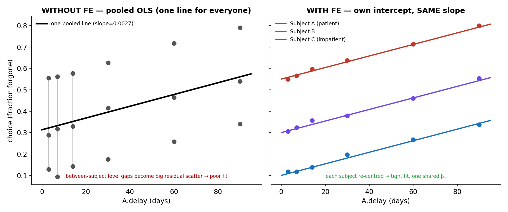
feols(... | id)does not average 178 separate slopes. It demeans: for each subject it subtracts that subject's own mean ofchoice,A.delay,A.payment— annihilating the intercept and every time-invariant trait — then runs one OLS on the re-centred data. So is identified purely from within-subject variation (how your own choice moves as your own delay changes), pooled into a single estimate.feols(... | factor(id))(fe1) instead prints all 178 dummy intercepts and you cluster the SEs by hand; the two give identical slopes and clustered SEs — fe2 is just the tidy readout that absorbs the intercepts.
Without FE, the same data looks like this — one pooled line ignores who each point belongs to, so the between-subject level gaps explode into residual scatter (left); FE re-centres each subject and the fit tightens onto parallel lines with one shared slope (right):
Part B — Does lower income cause higher choice? [Q2, 40 pts]
Outcome still continuous (
choice). The colleague's model addsincome: Worry: unobserved time preferences are correlated with income →incomeendogenous.
Q2a — Causal diagram for income endogeneity [15 pts]
AnswerA subject's unobserved time preferences live in the error . They affect choice directly (impatient people forgo more future money) and they affect income (e.g. impatient people save/invest less, earning less). So
incomeis correlated with — a violation of exogeneity () → endogeneity, and OLS on is biased.A.delayandA.paymentare randomly assigned by the researcher, so they are unaffected by income or preferences (though they still causechoice).
graph LR
    u["u = unobserved time preferences"] --> income["income"]
    u --> choice["choice"]
    income --> choice
    x["A.delay, A.payment (randomised)"] --> choice
    class u,income,choice,x internal-link;
    linkStyle 0,1 stroke:#c0392b,stroke-width:2px;
Hand-drawable version (exam practice)You must draw this DAG in the exam. Here it is as an editable Excalidraw canvas — open it and redraw until the structure is automatic. The red node
ufeeding two arrows (intoincomeandchoice) is what makesincomeendogenous.
Q2b — IV / 2SLS estimate [10 pts]
Instruments: hsheadnowork and avg.vilg.rainfall (both from the 2002 survey). Two instruments for one endogenous regressor → overidentified.
First stage — Dep. var.: income:
                   Estimate   Std. Error  t value    Pr(>|t|)
(Intercept)        -3.155679    2.162945   -1.459    0.1447
avg.vilg.rainfall   0.016315    0.001370   11.913    < 2.2e-16 ***
hsheadnowork      -13.253520    2.046885   -6.475    1.13e-10 ***
A.delay            ~0           0.012284    ~0        1.0000
A.payment          ~0           0.0000038   ~0        1.0000
---
F-test (1st stage): stat = 97.0, p < 2.2e-16
Second stage — Dep. var.: choice:
              Estimate     Std. Error   t value   Pr(>|t|)
(Intercept)   0.467936     0.024722     18.928    < 2.2e-16 ***
fit_income   -0.004901     0.001069     -4.583    4.80e-06 ***
A.delay       0.002728     0.000183     14.900    < 2.2e-16 ***
A.payment    -2.12e-07     5.09e-07     -3.732    1.94e-04 ***
---
Wu-Hausman: stat = 15.0, p = 1.08e-4    Sargan: stat = 9.603, p = 0.00194
Answer — the colleague is rightLook at
fit_incomein the second stage: , statistically significant (). The sign is negative: a 1-million-VND fall in income raiseschoiceby ≈ 0.005, i.e. the subject will forgo about 0.5% more of the future payment. So lower income does cause a stronger preference for money today — the colleague's suspicion is confirmed.
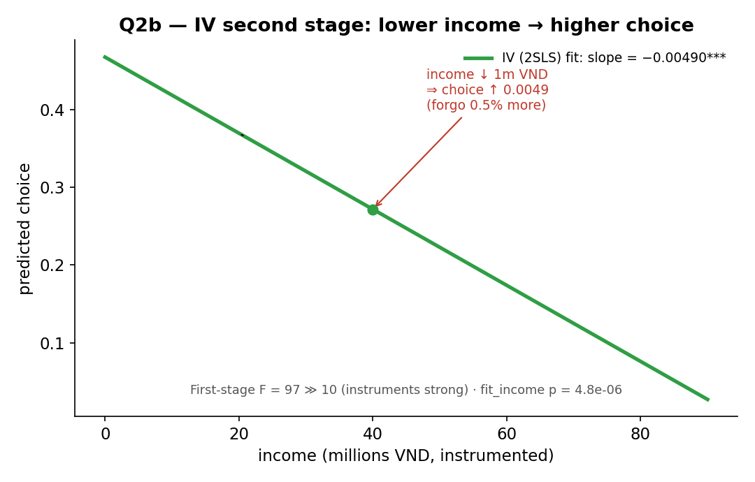
Reading the figure. The 2SLS line slopes down: instrumented income vs predicted choice. The strong first stage () means the instruments inject plenty of exogenous variation in income, so this slope is well-identified.
Why we trust the first stageA valid 2SLS needs a strong first stage. Here the joint , so these are not weak instruments. The Wu–Hausman test also rejects (), confirming income really was endogenous and IV was needed over OLS.
Q2c — Validity & relevance of the two instruments [15 pts]
Answer — Relevance ✅ (testable)Relevance requires the instruments to move
income() — and we can test it directly in the first stage. Both clear the bar at 5%:avg.vilg.rainfall(, positive — wetter villages are richer) andhsheadnowork(, negative — a household head unable to work means lower income). Joint confirms relevance. Both were measured in the same 2002 survey as income, which is why they predict it well.
Answer — Validity ✅ (argued, not tested)Validity (the exclusion restriction) requires the instruments to be uncorrelated with the error — to affect
choiceonly throughincome. We can't prove this, but the timing makes a strong case: the instruments are from 2002, the choices were made in 2005. Whether a household head couldn't work for 7 days in 2002, or how much rain fell in 2002, has no plausible direct channel to a money-vs-time choice three years later — except through its effect on income. So the exclusion restriction is credible.
Subtlety the official answer skips — the Sargan test actually rejectsBecause the model is overidentified (2 instruments, 1 endogenous regressor), validity is partially testable via the Sargan overidentification test in the output. Here Sargan , , so we reject the joint null that both instruments are valid. The honest reading: at least one instrument may violate the exclusion restriction (e.g. rainfall could affect current liquidity/consumption directly, not only via 2002 income). The conceptual timing argument is the expected exam answer, but a careful student notes the Sargan flag. (The test assumes ≥1 instrument is valid; it can't tell us which one fails.)
Part C — Does a higher Plan A payment change P(always pick today)? [Q3–Q4]
Outcome
today.alwaysis binary → LPM with robust SEs.
Q3 — Effect of A.payment on today.always [10 pts]
OLS estimation, Dep. var.: today.always   (Std-errors: Heteroskedasticity-robust)
              Estimate     Std. Error   t value   Pr(>|t|)
(Intercept)   0.208981     0.017323     12.064    < 2.2e-16 ***
A.delay       0.003093     0.000271     11.403    < 2.2e-16 ***
A.payment    -2.68e-07     8.19e-08     -3.276    0.00107   **
Answer — yes, a higher payment lowers P(always pick today)The coefficient on
A.paymentis , statistically significant (). Reading it as an LPM: raising Plan A by 30,000 VND (one step on the payment grid) changes P(always choose Plan B today) by , i.e. −0.8 percentage points. A bigger future prize makes subjects less likely to grab the immediate cash every time — exactly as economic intuition predicts.
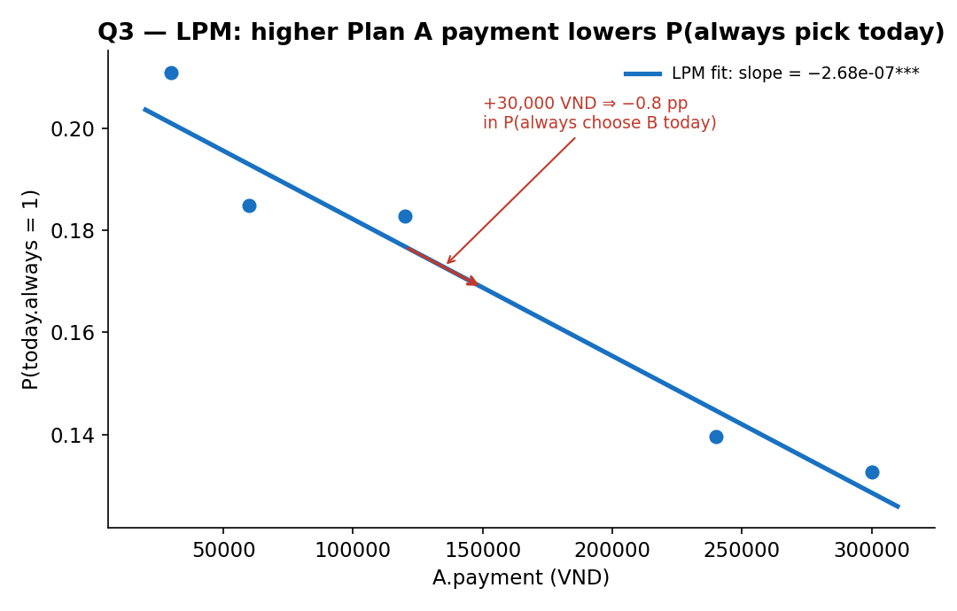
Reading the figure. The downward LPM line is P(today.always=1) against A.payment; the orange arrow shows the +30,000 → −0.8 pp reading. The fitted value is a predicted probability — the LPM interpretation.
Easy aside (don't forgetA.delay)
A.delayis also significant and positive (, ): a longer delay raises the probability of always taking money today. Same story as Part A, now on the binary margin — consistent evidence that delay drives impatience.
Tiny number-check discrepancyThe official write-up quotes the
A.paymentp-value as 0.000975; the printed output reads 0.00107. Either way it's far below 0.05, so the conclusion (significant, negative) is unchanged.
Q4 — DiD robustness check: did the typhoon warning affect choices? [25 pts]
Backstory: in village N3 a typhoon alarm interrupted the session right after round 6. Nearby village N4 (same province) ran a few days earlier with no interruption. The colleague runs a difference-in-differences check:
Q4a — Define the groups & write the R code [15 pts]
Answer
- Treatment group = subjects in N3 (the village hit by the typhoon warning). Control group = subjects in N4.
- Pre-period = rounds 1–5 (before the alarm). Post-period = rounds 6–15 (after).
effectis the DiD interaction (group × period); its coefficient is the typhoon effect.
# Treated = N3 (the typhoon village); control = N4.
# Post = from round 6 onward (the alarm hit right after round 6).
panel.data$treatment = as.numeric( panel.data$village == "N3" )
panel.data$post      = as.numeric( panel.data$round  >= 6  )
panel.data$effect    = panel.data$treatment * panel.data$post   # DiD interaction

DID1 = lm(today.always ~ treatment + post + effect, data = panel.data,
          subset = panel.data$village %in% c("N3", "N4"))
summary(DID1)
Why this coding is the one to reproduceEach variable means exactly what it says:
treatment= the group that received the shock (N3),post= the periods after it (rounds 6–15), andeffect = treatment × post. With this setup a positiveeffectwould say the typhoon raisedtoday.always, a negative one that it lowered it — the sign reads straight off. The DiD estimate you interpret is always the interaction , never the two main effects (which just set the group gap and the common time trend).
Q4b — Read the output [10 pts]
              Estimate   Std. Error  t value   Pr(>|t|)
(Intercept)   0.21000    0.04590      4.575    4.76e-06 ***
treatment     0.05666    0.06215      0.912    0.362
post          0.11500    0.05622      2.046    0.041    *
effect       -0.03583    0.07612     -0.471    0.638
Answer — no, the typhoon warning had no detectable effectRead the interaction
effect= — the DiD estimate. It is not statistically significant (), so we cannot reject that the typhoon warning had zero effect on choices. The colleague's robustness check passes — the interruption does not appear to have changed behaviour.(The main effects are just scaffolding:
post = +0.115is the common upward time trend both villages share — note rounds 6–15 use larger/longer Plan A offers — andtreatment = +0.057is N3's baseline gap above N4. Neither answers the research question; only the interaction does.)
type: diff-in-diff
control: 0.21,0.325
treatment: 0.26666,0.34583
controlName: N4 (control village)
treatmentName: N3 (typhoon warning)
periods: Pre (rounds 1–5),Post (rounds 6–15)
yLabel: mean today.always
decimals: 3
Reading the figure. N3 (treated) and N4 (control) both drift up from pre to post. The dashed line is N3's counterfactual under parallel trends (N3's pre-level + N4's change). The DiD is the gap between N3's actual post-point and that counterfactual — small (−0.036) and statistically indistinguishable from zero.
One-page recap (what each part tests)
| Q | Tool | Answer in one line |
|---|---|---|
| 1a | Baseline OLS + H-test | choice = β₀+β₁delay+β₂payment+u; test |
| 1b | OVB + serial corr. | Round is in the error → add it; then plain OLS SEs are fine |
| 1c | Individual FE + cluster | `feols(choice ~ delay+payment |
| 2a | Causal DAG | time prefs u → income & choice ⇒ income endogenous |
| 2b | 2SLS | fit_income = −0.0049*** ⇒ lower income → higher choice |
| 2c | Validity & relevance | relevant (1st-stage F=97); valid by 2002-vs-2005 timing — but Sargan rejects |
| 3 | LPM | A.payment = −2.68e-07** ⇒ +30k → −0.8 pp P(today.always) |
| 4a | DiD setup | treat=N3, control=N4; pre=rounds 1–5, post=6–15; effect=interaction |
| 4b | DiD inference | effect = −0.036 () ⇒ no typhoon effect |
Related Notes
- Foundational: Lec_04-Instrumental Variables · Lec_08-Fixed Effects in Panel Data · Lec_02-Linear Probability Model (LPM) · Lec_10-Difference-in-Differences
- Sister past papers: PP_02-Holdup Game & Bargaining (2023 Moed A) (the Moed A twin — LPM, DAGs, IV validity) · PP_01-Emotions & Risky Choice (Practice Exam) (FE, LPM vs probit, DiD, IV)
- Applied practice: PS_02-Fertility & Education (IV validity & 2SLS) · PS_04-Seatbelt Laws & Traffic Fatalities (panel FE & clustered SEs)
- Concepts: Instrumental Variables · Fixed Effects · Linear Probability Model · Difference-in-Differences
- Hub: Econometrics