
Practice Exam — Emotions & Risky Choice (Lab-in-Field)
Dataset: Lab-in-field emotion/lottery experiment — 243 subjects × 15 rounds
- #econometrics
- #past-paper
- #exam-prep
- #linear-probability-model
- #f-test
- #causal-diagram
- #omitted-variable-bias
- #fixed-effects
- #probit
- #marginal-effects
- #difference-in-differences
- #instrumental-variables
Practice Exam — Emotions & Risky Choice (Lab-in-Field)
Part of: Econometrics Practice Exam — Applied Econometrics, Dr. Aluma Dembo Key concepts: F-test, Linear Probability Model, Causal Diagram, Endogeneity, Omitted Variable Bias, Fixed Effects, Within Estimator, Probit Model, Marginal Effects, Difference-in-Differences, Instrumental Variables, Instrument Relevance, Instrument Validity Builds on: Lec_02-Linear Probability Model (LPM), Lec_03-Logit & Probit Models, Lec_04-Instrumental Variables, Lec_08-Fixed Effects in Panel Data
The Setup (read this first)
A researcher studies the effect of emotion and energy on risky choice. 243 subjects play 15 rounds of a lottery game on an app; before each round they self-report emotion (1 = sad … 7 = happy) and energy (1 = tired … 7 = energetic).
| Variable | Meaning |
|---|---|
chose.B |
=1 if subject chose the risky Lottery B in round (the binary outcome) |
diff.E |
Expected payout of B − Expected payout of A in round (varies by round only) |
emotion, energy |
Self-reported emtotion / energy, 1–7 |
dayofweek, timeofday |
When the choice was made (rounds were randomised across the week) |
celsius, sleep |
Outdoor temperature & hours slept the night before |
The single most important observationThe outcome
chose.Bis binary. So everylm/feols/anovain this exam is a Linear Probability Model — coefficients are changes in the probability of choosing B, measured in percentage points. Spotting this immediately tells you how to interpret every coefficient and why robust/clustered SEs appear. See Lec_02-Linear Probability Model (LPM).
This is a panel: each subject is observed over rounds → opens the door to Fixed Effects.
Q1 — Joint test, DAG, and endogeneity [20 pts]
1a — The anova() test
Two nested models (OLS2 is OLS1 with ):
anova(ols1, ols2) runs an F-test of against at least one . From the output: on and df, .
AnswerReject . Because (indeed astronomically small), at least one of
emotion,energyhas a non-zero effect onchose.B.What it tells us about OLS2: since emotion and/or energy genuinely belong in the model but are left out of OLS2, they get absorbed into OLS2's error term. OLS2 is therefore an under-specified model whose error contains a systematic (non-random) component.
Where the F-stat comes fromThe restricted model OLS2 has a larger residual sum of squares (RSS) than the unrestricted OLS1 (RSS). The test asks whether dropping the two regressors costs "too much" fit: with restrictions. Large ⇒ the variables matter ⇒ reject. (See Hypothesis Testing.)
1b — Updated causal diagram
The colleague's worry: intrinsic risk preferences are an individual, time-invariant trait that makes people both more optimistic/energetic and more likely to pick the risky lottery. That makes risk.preferences a common cause (confounder) of emotion, energy and the choice.
graph TD
    diffE["diff.E_t"] --> choseB["chose.B_it"]
    emotion["emotion_it"] --> choseB
    energy["energy_it"] --> choseB
    risk["risk.preferences_i (unobserved)"] --> emotion
    risk --> energy
    risk --> choseB
    u["u_it"] --> choseB
    class diffE,emotion,energy,choseB,risk internal-link;
The new node risk.preferences has arrows into emotion, energy, and chose.B — it is the backdoor path that contaminates the emotion→choice and energy→choice relationships. See Causal Diagram, Endogeneity.
Hand-drawable version (exam practice)The Mermaid diagram above renders for reading, but in an exam you'd draw this. Here's the same DAG as an editable Excalidraw canvas — open it, redraw it freehand a few times until the confounder structure is muscle memory. Red arrows = the backdoor path you must be able to spot and explain.
1c — Where do risk preferences show up in OLS1, and what does it mean for ?
OLS1 does not include a risk.preferences regressor (it's unobserved), so it sits inside the error term . But risk preferences also drive emotion and energy → so the regressors are correlated with the error:
ConsequenceThis is textbook Endogeneity caused by an omitted common cause — i.e. Omitted Variable Bias. and are therefore biased and do not measure the causal effect of emotion/energy on choice; they partly pick up the effect of the omitted risk preferences. The estimates conflate "happier people choose B" with "risk-lovers are both happier and choose B."
Q2 — Fixed effects & probit [20 pts]
R fits an individual fixed-effects LPM (fe1) with SEs clustered by subject ID:
fe1 = feols(chose.B ~ diff.E + energy + emotion | ID, mydata) # 243 individual FEs
| Term | Estimate | Std. Error (clustered) | ||
|---|---|---|---|---|
diff.E |
0.0267 | 0.00089 | 30.05 | <2e-16 |
energy |
0.0297 | 0.00965 | 3.08 | 0.00233 |
emotion |
0.0384 | 0.00720 | 5.33 | 2.27e-07 |
2a — Why FE1 over OLS1?
Intrinsic risk preferences are time-invariant (they don't change over the 5-day study). An Individual Fixed Effect is exactly a per-subject intercept that absorbs every characteristic of that is constant over time — including their unobserved risk preferences.
AnswerBy including individual fixed effects, FE1 demeans each subject's data (Within Estimator / Demeaning) and identifies purely from Within Variation — how a person's own emotion/energy fluctuates round to round. Because risk preferences are fixed within a person, they are differenced out, so the confounder from Q1 is controlled and the endogeneity it caused is removed. Clustering SEs by
IDaccounts for the repeated observations per subject. See Lec_08-Fixed Effects in Panel Data.
Why the fixed effect mechanically absorbs risk preferencesWrite the model with a per-subject intercept (this is what
| IDadds — one intercept per subject): The estimator subtracts each subject's own average from every variable (the within / demeaning transform). For any quantity that is constant within a subject — likerisk.preferences— its value equals its own mean, so it subtracts to zero: That's the whole trick: the confounder doesn't need to be measured — anything time-invariant for a subject is annihilated by demeaning and can no longer sit in the error correlating with emotion/energy.Why
ID(the subject) and not, say,dayofweek? Put the fixed effect at the level where the confounder is constant. Risk preference varies between people but is fixed within a person across the 15 rounds — so subject-level (ID) effects kill it. Day or round effects wouldn't: risk preference isn't constant within a day. Rule: FE at the level of the omitted variable you're trying to remove.
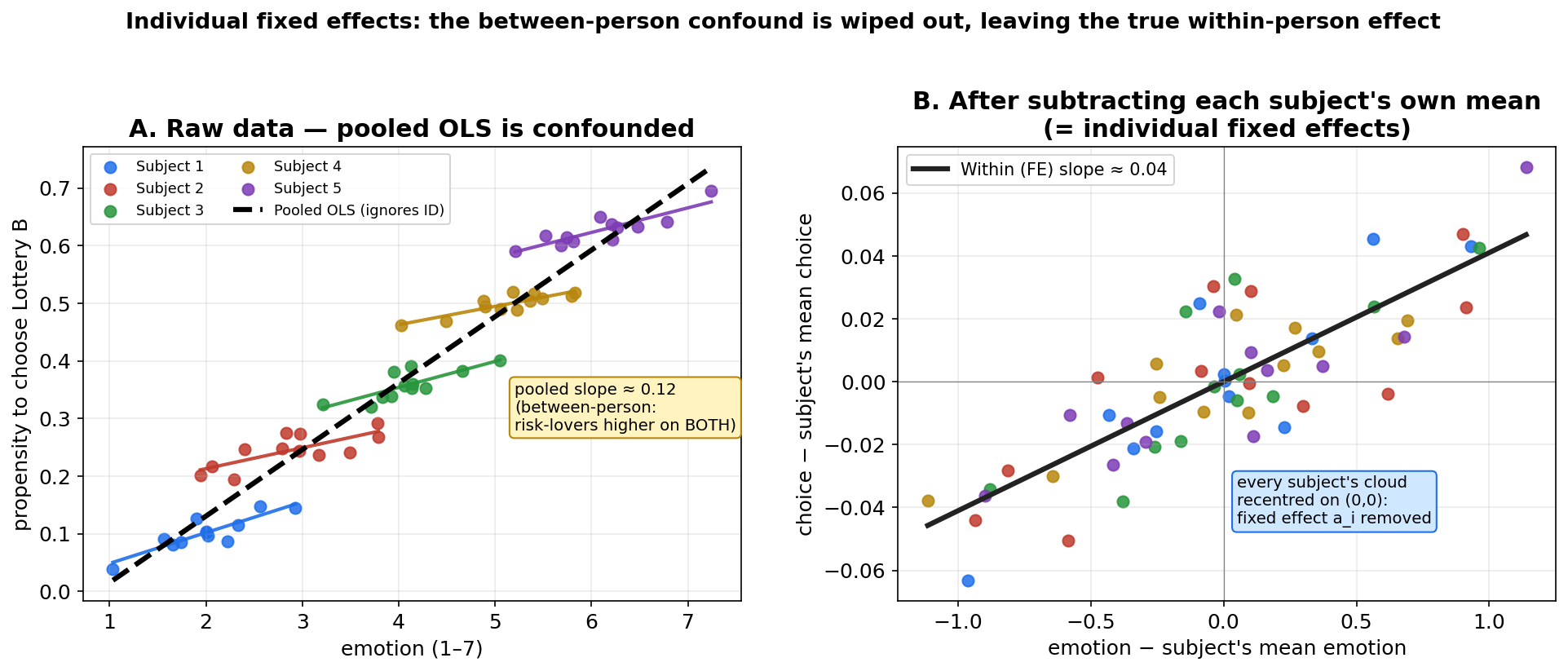
Reading the figure. Left: each subject is one colour; their points cluster because each has a different baseline (their fixed effect ). Risk-lovers sit high on both axes, so the pooled OLS line (dashed, slope ≈ 0.12) is steep — it's mostly measuring the between-person confound, not causation. Right: after subtracting each subject's own mean, every cloud recentres on — the differences vanish — and the remaining within slope (≈ 0.04) is the true effect of a person's emotion changing. That within slope is what FE1 reports, and it matches the exam's emotion coefficient (0.038).
2b — Interpreting the FE coefficients (with significance at α = 5%)
Still an LPM, so coefficients are in percentage points, now interpreted relative to the subject's own average:
emotion= 0.0384: a one-point rise in emotion (above the subject's own mean) raises the probability of choosing B by ≈ 3.84 pp. Significant: ✓ (also ).energy= 0.0297: a one-point rise in energy raises by ≈ 2.97 pp. Significant: ✓ ().
AnswerBoth coefficients are positive and statistically significant at the 5% level. Within-person, happier and more energetic moments are associated with more risk-taking, by roughly 3.8 pp and 3.0 pp per scale point respectively.
2c — The probit model
probit = glm(chose.B ~ diff.E + emotion + energy, mydata, family = binomial(link = "probit"))
| Term | Estimate | ||
|---|---|---|---|
(Intercept) |
−1.722 | −18.59 | <2e-16 |
diff.E |
0.0786 | 26.39 | <2e-16 |
emotion |
0.229 | 10.63 | <2e-16 |
energy |
0.215 | 8.89 | <2e-16 |
Answerand , both highly significant → higher emotion and higher energy each increase the probability of choosing B (we can read the sign and significance).
But we cannot read the magnitude directly. In a Probit Model the coefficients are not the Marginal Effects: the effect on the probability is , which depends on where you evaluate it. So unlike the LPM, "0.229" is not "22.9 pp." To get a marginal effect you must compute at a chosen point (e.g. the mean). See Lec_03-Logit & Probit Models.
type: binary-curves
mode: probit-slopes
The probit S-curve is steepest in the middle and flat at the tails: the same one-point rise in emotion moves the probability a lot near but barely at all near 0 or 1. That changing slope is the marginal effect . The grey LPM line has one constant slope — which is exactly why an LPM coefficient is its marginal effect while a probit coefficient is not.
Exam contrast to rememberLPM coefficient = the marginal effect (constant, in pp). Probit/logit coefficient = direction & significance only; marginal effect is non-constant. This single distinction is worth easy marks.
Q3 — Difference-in-Differences [30 pts]
Builds on: Lec_10-Difference-in-Differences — this question is the lecture's 2×2 design applied to the exam shock. Same logic as the Card & Krueger worked example.
86 of the 243 subjects sat an econometrics final on Wednesday morning, just before that day's task. On Wednesday, exam-takers reported mean emotion 2.53 vs 3.11 for non-takers — the exam was an emotional shock. We use it as a natural experiment via Difference-in-Differences to recover the Average Treatment Effect on the Treated (the effect on those who actually sat the exam).
3a — Treatment/control groups and pre/post periods
Answer
- Treatment group: all observations of subjects who took the exam (86 subjects).
- Control group: all observations of subjects who did not take the exam (157 subjects).
- Pre-period: observations before Wednesday (Mon–Tue).
- Post-period: observations from Wednesday (after the exam) onward — Wed–Fri. (Also acceptable: drop Wednesday and use Thu–Fri, or compare Wed-morning vs Thu-evening.)
The exam can't be randomly assigned, so we don't compare raw levels — we compare the change in each group, which differences out fixed group gaps. Note these are repeated cross-sections across rounds, which is all DiD needs (no panel required — see Lec 10).
3b — The DiD estimate
Sample means of chose.B:
| Pre-period | Post-period | |
|---|---|---|
| Control | 0.52 | 0.47 |
| Treatment | 0.41 | 0.43 |
Answer: DiD ATE = 0.07The control group's choices drifted down 0.05 over the week (a common time trend). The treatment group went up 0.02. Netting out the common trend, taking the exam is associated with a +0.07 (7 pp) change in the probability of choosing B, relative to what would have happened absent the exam.
type: diff-in-diff
control: 0.52,0.47
treatment: 0.41,0.43
controlName: Control (no exam)
treatmentName: Treatment (took exam)
periods: Pre (Mon–Tue),Post (Wed–Fri)
yLabel: P(chose lottery B)
decimals: 2
The dashed red line is the counterfactual: where the treatment group would have ended up (0.36) if it had followed the control group's trend. The vertical gap between the actual treatment endpoint (0.43) and that counterfactual (0.36) is the DiD estimate, 0.07.
Equivalent calculation (cross-difference order)Same answer — DiD is symmetric in the order you difference. (Only one calculation needed on the exam.)
Same answer via the regression form (if asked for significance)The by-hand 0.07 is exactly the interaction coefficient in where = post-period dummy and = exam-taker dummy. Running this as a regression is how you'd get a standard error / significance on the 0.07 — which the sample-average method can't give. See Lec 10: DiD as a regression.
Identifying assumption — don't forget thisDiD is only causal under parallel trends: absent the exam, treatment and control groups'
chose.Bwould have moved by the same amount. We can't test it directly, but the −0.05 control drift is the counterfactual trend we're subtracting off. The lecture lists three validity conditions: (1) no other shock hits the control group around Wednesday, (2) takers and non-takers are otherwise comparable, and (3) parallel pre-trends. Here (1) is the real worry — Wednesday is mid-week, and anything else that shifted choices that day (fatigue, other classes) would contaminate the estimate.
Q4 — Instrumental Variables [30 pts]
emotion and energy are endogenous (Q1). The colleague proposes two instruments: celsius (outdoor temperature) and sleep (hours slept). Two endogenous regressors ⇒ we need (at least) two instruments. See Instrumental Variables, Two Stage Least Squares.
4a — R pseudo-code
iv1 = feols(chose.B ~ diff.E | emotion + energy ~ sleep + celsius,
            data = mydata, se = "hetero")
How to read thefixestIV formula
chose.B ~ diff.E= outcome and the exogenous/included regressor; after the|,emotion + energy ~ sleep + celsiussays "instrument the two endogenous regressors on the left with the two instruments on the right." The First Stage regresses each of emotion and energy onsleep,celsius(+diff.E); the second stage uses the fitted values.
4b — Relevance and validity
The correlation matrix:
| chose.B | emotion | energy | sleep | celsius | |
|---|---|---|---|---|---|
| emotion | 0.204 | 1.000 | 0.312 | −0.036 | 0.793 |
| energy | 0.189 | 0.312 | 1.000 | 0.718 | −0.011 |
| sleep | 0.030 | −0.036 | 0.718 | 1.000 | −0.007 |
| celsius | 0.065 | 0.793 | −0.011 | −0.007 | 1.000 |
Relevance — satisfiedInstrument Relevance requires . Here
celsiusis strongly correlated with emotion () andsleepis strongly correlated with energy (). Conveniently each instrument loads on a different regressor (celsius–energy ≈ 0, sleep–emotion ≈ 0), so the pair jointly identifies both. These are strong, not Weak Instruments.
Validity — an assumption, not something the table can proveInstrument Validity (the exclusion restriction) requires and . Since is unobserved, the correlation table cannot confirm validity — you must argue it. Reasonable cases either way:
- Threat: temperature might affect choices directly (heat/discomfort changing decision-making), not only through emotion → exclusion violated. Likewise sleep may affect cognition/attention beyond just "energy" → violated.
- Defence: if the only channel from weather→choice is mood, and from sleep→choice is energy, the instruments are valid.
(The exam accepts any well-reasoned validity discussion.)
One-page recap (what each part tests)
| Q | Tool | Answer in one line | ||
|---|---|---|---|---|
| 1a | anova = _Econometrics Concepts#F-test |
Joint significance of nested models | Reject ; omitted vars sit in OLS2's error | |
| 1b | _Econometrics Concepts#Causal Diagram | Draw a confounder | risk.preferences → emotion, energy, choice |
|
| 1c | _Econometrics Concepts#Omitted Variable Bias | Endogeneity from omitted common cause | biased, not causal | |
| 2a | _Econometrics Concepts#Fixed Effects | Why FE beats OLS here | absorbs time-invariant risk prefs | |
| 2b | _Econometrics Concepts#Linear Probability Model | Interpret LPM coefs + significance | +3.84 pp, +2.97 pp; both sig. at 5% | |
| 2c | _Econometrics Concepts#Probit Model | Coef ≠ _Econometrics Concepts#Marginal Effects | Marginal Effects | Read sign only; magnitude needs |
| 3 | _Econometrics Concepts#Difference-in-Differences | Compute DiD ATE | ||
| 4a | _Econometrics Concepts#Two Stage Least Squares | Write IV in fixest |
feols(y ~ x | endog ~ instruments) |
|
| 4b | _Econometrics Concepts#Instrument Relevance | Instrument Validity | Judge instruments | Relevant (ρ≈0.79, 0.72); validity is unprovable assumption |
Related Notes
- Foundational: Lec_02-Linear Probability Model (LPM) · Lec_03-Logit & Probit Models · Lec_04-Instrumental Variables · Lec_08-Fixed Effects in Panel Data
- Applied practice: PS_04-Seatbelt Laws & Traffic Fatalities (fixed effects & DiD) · PS_02-Fertility & Education (IV & validity)
- Concepts: F-test · Endogeneity · Omitted Variable Bias · Within Estimator · Marginal Effects · Parallel Trends Assumption
- Hub: Econometrics