
2023 Moed A — Holdup Game & Bargaining Behavior
Dataset: holdup — 103 Buyer–Seller pairs, Swedish lab experiment (Control/Promises/Threats)
- #econometrics
- #past-paper
- #exam-prep
- #linear-probability-model
- #dummy-variables
- #logit
- #marginal-effects
- #causal-diagram
- #endogeneity
- #omitted-variable-bias
- #instrumental-variables
- #endogenous-selection
2023 Moed A — Holdup Game & Bargaining Behavior
Part of: Econometrics Final Exam 2023 — Moed A — Applied Econometrics, Dr. Aluma Dembo Key concepts: Linear Probability Model, Dummy Variables, Robust Standard Errors, Hypothesis Testing, Logit Model, Marginal Effects, Maximum Likelihood Estimation, Causal Diagram, Endogeneity, Omitted Variable Bias, Instrumental Variables, Instrument Validity, Instrument Relevance, Endogenous Selection, Ultimatum Game Builds on: Lec_02-Linear Probability Model (LPM), Lec_03-Logit & Probit Models, Lec_04-Instrumental Variables
The Setup (read this first)
A Swedish lab experiment runs the Holdup game — the ultimatum game with an extra trust stage at the front. Each of 103 Buyer–Seller pairs is randomly assigned to one of three communication conditions:
| Treatment | N | What's different |
|---|---|---|
| Control | 40 | No communication |
| Promises | 30 | Buyer messages the Seller before Stage 1 (can promise a generous offer) |
| Threats | 33 | Seller messages the Buyer before Stage 2 (can threaten to reject low offers) |
The game runs in three stages, and each stage produces one variable:
- Stage 1 — Seller chooses Invest / Don't invest →
invest(binary) - Stage 2 — Buyer proposes a split out of 100 →
offer(0–100, NA if no invest) - Stage 3 — Seller Accepts / Rejects →
accept(binary, NA if no invest)
The single most important observationTwo of the three outcomes are binary:
invest(Part A) andaccept(Part C). So every regression on those is a Linear Probability Model — coefficients are changes in a probability, and you must use heteroskedasticity-robust SEs.offer(Part B) is continuous, so model [2] is ordinary OLS. Spotting which is which tells you immediately how to read every coefficient and which SEs are needed.
The second thing that unlocks the paper — the sequential structure is the causal graphBecause the stages happen in order, earlier choices cause later ones. The Seller's threat affects the Buyer's offer and the Seller's own acceptance; the Buyer's "fairness type" drives both what they promise and what they offer. That sequential structure is exactly why Parts B and C hinge on endogeneity and causal diagrams, not just regression mechanics.
Every regressor here is a dummy with Control as the omitted base group, so every treatment coefficient reads as "difference versus Control."
Part A — Do promises affect the decision to invest? [Q1–Q2]
Uses the full dataset (all 103 pairs). Outcome
investis binary → LPM and logit.
Q1a — Interpreting and answering RQ (A) [20 pts]
AnswerBoth coefficients are differences in the probability of investing relative to the Control group (the omitted dummy):
- = change in P(invest) for a promises-treatment pair vs control.
- = change in P(invest) for a threats-treatment pair vs control.
The research question is specifically about promises, so we test against . Rejecting means promises shift the probability of investing.
Why the coefficients are the group meansWith only dummies and control omitted, the fitted values are exactly the cell means: , and . Check against the data table: control invest rate , promises , threats — these reproduce in the output below.
Q1b — R pseudo-code [part of Q1]
lpm = feols(invest ~ promises + threats, data = holdup, se = "hetero")
AnswerBecause
investis binary this is an LPM, whose errors are inherently heteroskedastic (the variance depends on ). So we must request heteroskedasticity-robust standard errors (se = "hetero") or the inference is wrong.
Q1c — Reading the output
              Estimate Std. Error t value  Pr(>|t|)
(Intercept)   0.350000   0.076538  4.57287 1.3809e-05 ***
promises      0.183333   0.120014  1.52760 1.2977e-01
threats       0.286364   0.114371  2.50381 1.3904e-02 *
Answer — promises have no detectable effectThe
promisescoefficient is not statistically significant: (also ). So even though the point estimate is +18.3 pp, we cannot distinguish the promises group's investment probability from control. Conclusion: promises do not significantly affect the decision to invest.(Aside:
threatsis significant at 5%, — but that's not what RQ (A) asks.)
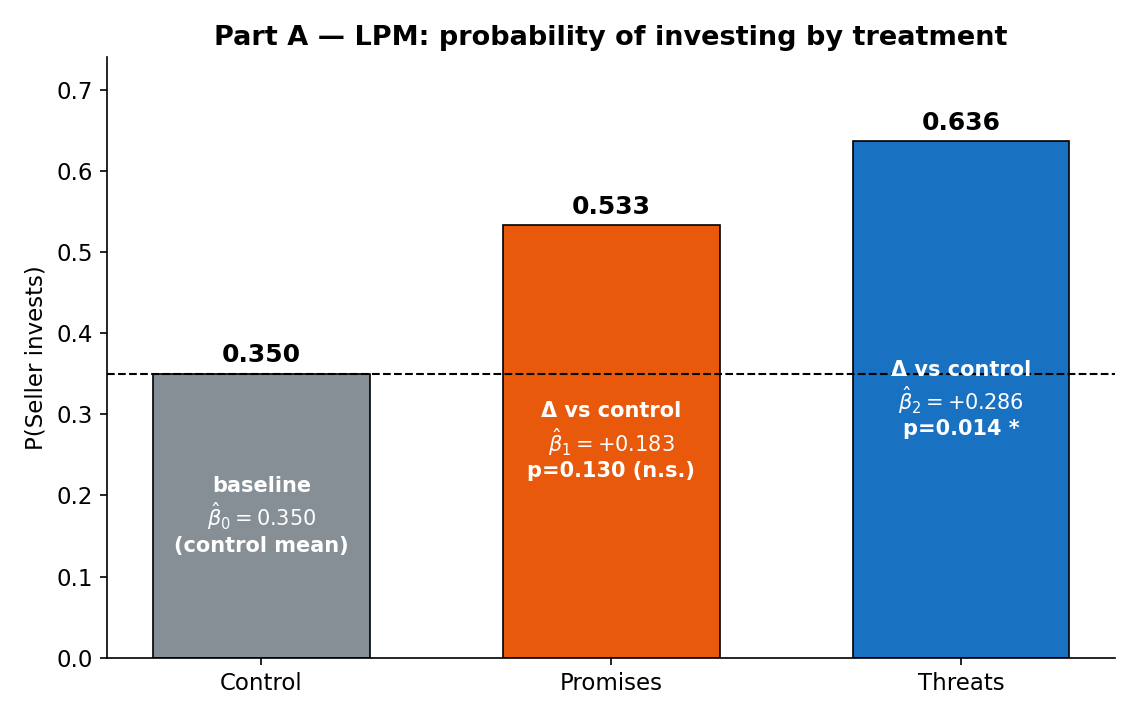
Reading the figure. Each bar is a group's invest rate, which equals the LPM's fitted value. The intercept is the control mean (0.350); each treatment coefficient is the gap up to that treatment's bar. The promises gap (+0.183) looks sizeable but its standard error is wide (0.120) → not significant. The threats gap (+0.286) is the one that clears the 5% bar.
Easy trapA non-significant coefficient does not mean "promises have zero effect." It means we can't reject zero at this sample size (only 30 promises pairs). With a positive point estimate and a wide SE, the honest statement is "no statistically significant effect," not "no effect."
Q2a — The logit version [20 pts]
Answerwhere is the logistic CDF and collects the regressors. Unlike the LPM, squashes the linear index into , so predicted probabilities are always valid. Estimated by maximum likelihood. See Lec_03-Logit & Probit Models.
Q2b — Which line of code gives the marginal effect?
coef(logit)                                          # option 1
dlogis( coef(logit) * averages )                     # option 2
coef(logit)*dlogis( sum( coef(logit) * averages ) )  # option 3  ✅
coef(logit)*dnorm(  sum( coef(logit) * averages ) )  # option 4
coef(logit)*plogis( sum( coef(logit) * averages ) )  # option 5
Answer — option 3In logit the coefficient is not the marginal effect. The effect of
promiseson P(invest) is i.e. the logistic density evaluated at the linear index (using the sample-average 's), times the coefficient. Mapping to the code:
- the index is
sum(coef(logit) * averages)— a single number;dlogis(...)is the logistic density (the right one —dnormwould be probit,plogisis the CDF not the density);- multiplying by
coef(logit)gives the marginal effect for each variable.Option 3 is the only one that computes . (Option 2 wrongly multiplies element-wise inside
dlogisinstead of summing to the index; options 4–5 use the wrong function.)
How to eliminate the distractors fast"Marginal effect of a logit = density × coefficient." The density of a logistic variable is
dlogis→ kills option 4 (dnorm) and option 5 (plogis, a CDF). The argument must be the scalar indexsum(coef·avg)→ kills option 2 (which feeds a vector intodlogis). What's left is option 3.
Q2c — Advantage of logit over the LPM
AnswerThe logit's fitted probabilities are bounded in because the logistic CDF asymptotes at 0 and 1. The LPM is OLS on a binary outcome, so its linear fitted values are unbounded and can fall below 0 or above 1 — nonsensical for something we interpret as a probability. (Part C, Fig below, shows the LPM line literally crossing .) See Lec_03-Logit & Probit Models.
Part B — How do threats & promises affect the offer? [Q3]
Uses only pairs whose Seller invested (the 51 pairs with a non-NA
offer). Outcomeofferis continuous → plain OLS.
Q3a — Reading the output at α = 5% and α = 10% [30 pts]
              Estimate Std. Error t value  Pr(>|t|)
(Intercept)    48.571      6.055   8.022  2.04e-10 ***
promises       21.429      8.291   2.584  0.0128   *
threats        14.762      7.817   1.888  0.0650   .
Residual standard error: 22.66 on 48 degrees of freedom
  (52 observations deleted due to missingness)
Answer
- Promises: . Significant at both 5% and 10% (). Being in the promises treatment raises the Buyer's offer by ≈ 21.4 SEK relative to control.
- Threats: . Not significant at 5%, but significant at 10% (). Being in the threats treatment raises the offer by ≈ 14.8 SEK relative to control (weaker evidence).
- Both communication channels increase the offer, with promises raising it slightly more. Caveat: we cannot test whether the difference between the two effects (21.4 vs 14.8) is significant from this output alone.
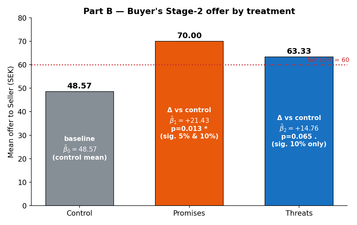
Reading the figure. Each bar is a treatment's mean offer (= the model's fitted value); the intercept is the control mean (48.57), below the "fair" 60/40 split. Communication pushes offers above 60: promises to 70.0, threats to 63.3. The labels carry each coefficient and its significance tier so you can see at a glance which clears 5% (promises) and which only clears 10% (threats).
Why we condition on "invested only"
offeris NA whenever the Seller didn't invest, so the 52 non-investing pairs drop out automatically — note "52 observations deleted due to missingness", leaving used (). This is a selected subsample (only pairs that reached Stage 2), which is the seed of the selection worry that returns in Part C.
Q3b — Why promise.made is endogenous (don't add it) [part of Q3]
A new variable promise.made = the amount the Buyer promised before Stage 1. It is tempting to add it to model [2], but it is endogenous.
AnswerThe Buyer's unobserved propensity for fairness/honesty drives both how much they promise (
promise.made) and how much they actually offer. Since that propensity is unobserved it lives in the error term . Thereforepromise.madeis correlated with — adding it violates the exogeneity assumption and produces omitted-variable bias in the treatment effect we care about. Keep it out of the model.
graph LR
    treat["assigned to promises"] --> pmade["promise.made (Stage 1)"]
    pmade --> offer["offer (Stage 2)"]
    fair["Buyer's fairness/honesty (unobserved → in u)"] --> pmade
    fair --> offer
    class treat,pmade,offer,fair internal-link;
The confounder fairness/honesty has arrows into both promise.made and offer — controlling for promise.made would open a backdoor path through that unobserved type. See Causal Diagram, Endogeneity.
Hand-drawable version (exam practice)In the exam you must draw this DAG. Here it is as an editable Excalidraw canvas — open it and redraw the confounder structure (red node feeding two arrows) until it's automatic. Red node = the unobserved type that makes
promise.madeendogenous.
Part C — Does the offer affect the Seller's acceptance? [Q4]
Uses only pairs whose Seller invested. Outcome
acceptis binary → LPM again.
Q4a — Endogeneity of offer and why threats isn't a valid IV [30 pts]
Consider the threats treatment, with the causal diagram: threats → Seller's threat; Seller's threat → offer; Seller's threat → accept; offer → accept.
Answer (i) —offeris endogenousThe Seller's threat (made before Stage 2) affects both the Buyer's
offerand the Seller's own likelihood of accepting in Stage 3. Because the threat is unobserved it sits in the error of model [3]; since it also drivesoffer, we get → endogeneity. OLS on model [3] is therefore biased.
Answer (ii) — threats-assignment fails as an IVA valid instrument must satisfy validity (the exclusion restriction): it may affect
acceptonly throughoffer. But assignment to threats reachesacceptthrough a second channel —threats → Seller's threat → accept— not routed through the offer. That extra path violates the exclusion restriction, so threats-assignment is not a valid instrument foroffer. (Its relevance is fine; it's validity that fails.)
graph LR
    treat["assigned to threats"] --> threat["Seller's threat (pre-Stage 2)"]
    threat --> offer["offer (Stage 2)"]
    threat --> accept["accept (Stage 3)"]
    offer --> accept
    class treat,threat,offer,accept internal-link;
Hand-drawable version (exam practice)The killer for the IV is the arrow
Seller's threat → acceptrunning parallel to the offer channel. An instrument is only valid if every path from it to the outcome passes through the endogenous regressor — here one doesn't.
Q4b — Reading the control-group estimate
            Estimate Std. Error t value Pr(>|t|)
(Intercept) 0.334126  0.156049   2.141  0.05348 .
offer       0.009297  0.002706   3.436  0.00493 **
Residual standard error: 0.3147 on 12 degrees of freedom
  (26 observations deleted due to missingness)
Multiple R-squared: 0.4959,  Adjusted R-squared: 0.4539
AnswerThe
offercoefficient is , significant at the 1% level (). Interpreting the LPM: a 10-SEK higher offer raises the probability the Seller accepts by ≈ 9.3 pp. So within the control group, more generous offers are accepted more often.
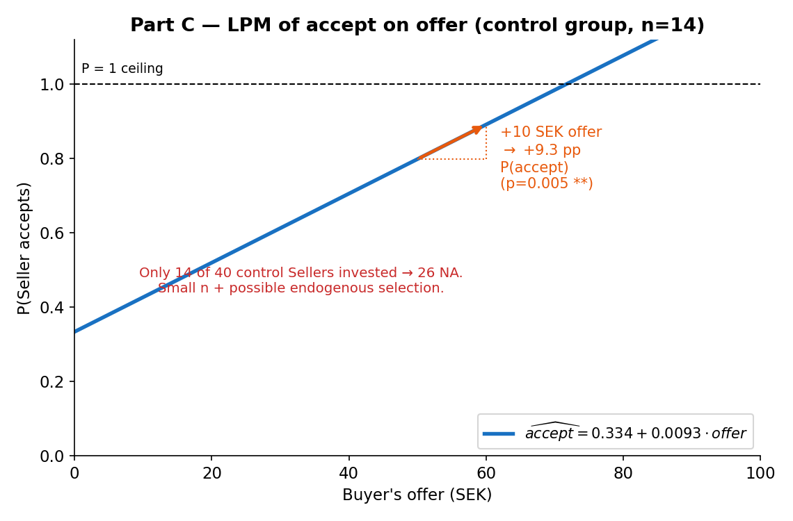
The fitted LPM line climbs at 0.93 pp per SEK; the orange step shows the +10 SEK → +9.3 pp reading. Note the line crosses at high offers — the LPM boundedness problem from Q2c made concrete.
What to be worried about — tiny, selected sampleThe regression runs on only 14 observations: of the 40 control pairs, in 26 the Seller didn't invest, so
accept/offerare NA and drop out. Two concerns:
- Tiny n (14) → imprecise, fragile estimates.
- Endogenous selection → the Sellers who chose to invest are not random. Something about them (e.g. a disposition to accept even small offers) may drive both their Stage-1 investment and their Stage-3 acceptance, biasing . We're estimating the offer→accept relationship on a self-selected subset, so it may not generalise.
One-page recap (what each part tests)
| Q | Tool | Answer in one line |
|---|---|---|
| 1a | Dummy interpretation | = P(invest) gap vs control; test |
| 1b | LPM + robust SE | feols(invest ~ promises + threats, se="hetero") |
| 1c | Inference | promises p=0.130 → no significant effect on investing |
| 2a | Logit | , = logistic CDF |
| 2b | Marginal effect | Option 3: via dlogis(sum(coef·avg)) |
| 2c | LPM vs logit | logit keeps ; LPM predictions unbounded |
| 3a | OLS on continuous offer |
promises +21.4 (sig 5%); threats +14.8 (sig 10% only) |
| 3b | OVB / DAG | fairness type → promise.made & offer ⇒ promise.made endogenous |
| 4a | IV validity | threat confounds offer→accept; threats-assignment has 2nd path ⇒ invalid IV |
| 4b | Endogenous selection | offer +9.3 pp/10 SEK (p=0.005) but n=14, self-selected |
Related Notes
- Foundational: Lec_02-Linear Probability Model (LPM) · Lec_03-Logit & Probit Models · Lec_04-Instrumental Variables
- Sister past paper: PP_01-Emotions & Risky Choice (Practice Exam) (same instructor — LPM/probit, DAGs, IV, DiD)
- Applied practice: PS_05-Labor Unions & Product Recalls (LPM & omitted-variable bias) · PS_02-Fertility & Education (IV validity & selection)
- Concepts: Linear Probability Model · Marginal Effects · Endogeneity · Instrument Validity · Endogenous Selection
- Hub: Econometrics