
Lookups with XLOOKUP and INDEX MATCH
- #excel-data-analysis
- #xlookup
- #index-match
- #lookup
- #approximate-match
- #pivot-table
Lookups with XLOOKUP and INDEX MATCH
Part of: Excel for Data Analysis Key concepts: XLOOKUP, Exact Match, Approximate Match, Match Mode, Spill Range, INDEX and MATCH, MATCH, INDEX, Lookup Table
SourceThis note is built from one class workbook,
feedback.xlsx, with six sheets:employees(200 rows, the main table),feedback(50 rows),Branches(16 rows),index&match(178 students with five exercise grades), and two pivot sheetsSheet2andSheet3. Everything below uses the real values and formulas in that file. Theemployeestable repeats the one from Lec_01-Sorting, Filters & Database Functions; only the new columnsfeedback,Bonus,Salary + BonusandArea, plus the lookup blocks under the table, are covered here.
1. The idea of a lookup
A lookup answers: "I know a key (an employee ID, a branch name, a salary). Go to another table, find that key, and bring back a related value." It replaces copy and paste, and it keeps working when the data changes.
Every lookup has four ingredients:
| Ingredient | Question it answers | Example in this workbook |
|---|---|---|
| Lookup value | What am I searching for? | the employee ID in A2 |
| Lookup array | Where do I search? (one column or row) | feedback!$A$2:$A$51 (the IDs) |
| Return array | What do I bring back? (same size as the lookup array) | feedback!$K$2:$K$51 (the scores) |
| Match type | Must it be identical, or may it fall in a range? | exact, or "next smaller" |
The workbook uses two families of tools: XLOOKUP (new, one function) and INDEX and MATCH (older, two functions combined, but more flexible for two-way lookups).
2. XLOOKUP
2.1 Syntax
The teacher's own note sits in cell I206, in plain words: "xlookup(what value do you want to look up, from which column are we looking it up from, what do we want this value to return,,0(give the exact value back),)". In Excel's formal terms:
=XLOOKUP(lookup_value, lookup_array, return_array, [if_not_found], [match_mode], [search_mode])
| Argument | Meaning | Required? |
|---|---|---|
lookup_value |
the key to find | yes |
lookup_array |
the column (or row) to search in | yes |
return_array |
the column (or row) to return from | yes |
if_not_found |
what to show instead of #N/A |
no (empty, as in ,,) |
match_mode |
0 exact, -1 exact or next smaller, 1 exact or next larger, 2 wildcard |
no (default 0) |
search_mode |
1 first to last (default), -1 last to first, 2 or -2 binary search |
no |
Reading the double comma
XLOOKUP(D206,A2:A201,J2:J201,,0,)has empty slots. An emptyif_not_foundmeans "just give me#N/Aif nothing matches", and the empty last slot means "default search direction". The commas must stay so that0lands in thematch_modeposition.
2.2 Worked example: one employee's details
A small input block sits under the data. You type an ID, and the formulas fetch the person.
| Cell | Content |
|---|---|
D205:G205 |
headers Employee ID, First name, Last name, Monthly Salary |
D206 |
10199 (typed) |
G206 |
=XLOOKUP(D206,A2:A201,J2:J201,,0,) returns 12213 |
E206 |
=XLOOKUP(D206,A2:A201,B2:C201,,0,) returns Hodaya and Levy |
Result row, exactly as in the workbook:
| Employee ID | First name | Last name | Monthly Salary |
|---|---|---|---|
| 10199 | Hodaya | Levy | 12213 |
The ID 10199 is in A2:A201 at row 200, so Excel reads the salary from the same row of J2:J201.
Why the first name and last name sit in two cells from one formula
E206has a two-column return array,B2:C201(first name and last name side by side). XLOOKUP returns both cells of the matched row, and Excel spills them intoE206andF206. You enter the formula once, inE206;F206is filled automatically. This is a Spill Range (stored in the file as an array formula overE206:F206).
Common mistake: arrays of different size
lookup_arrayandreturn_arraymust have the same number of rows (for a vertical lookup).A2:A201andJ2:J201both have 200 rows, so they line up. If one range is shifted by a row, every answer is silently wrong.
2.3 Looking up a computed value: MAX and the youngest employee
XLOOKUP is often chained with an aggregate. First compute the target, then look it up.
| Block | Formula | Result |
|---|---|---|
Highest salary, G210 |
=MAX(J2:J201) |
14967 |
Who earns it, E210 |
=XLOOKUP(G210,J2:J201,B2:C201,,0,) |
Pini Korinsky |
Youngest birth date, G213 |
=MAX(F2:F201) |
31039 (the date 23 December 1984) |
Who it is, D213 |
=XLOOKUP(G213,F2:F201,A2:C201,,0) |
10038 Keren Mizrahi |
Why MAX for the youngestDates are numbers (days since 1900), and a later birth date is a larger number. The largest birth date belongs to the youngest person. For the oldest you would use
MIN.
Notice D213 returns three columns (A2:C201 is ID, first name, last name), so the result spills across D213:F213. Here the number of spilled columns is chosen simply by how wide the return array is.
Exact match on a computed number
MAXreturns a value that exists in the column, so exact match (0) is safe. Looking up a number you calculated by division or rounding can fail with#N/Abecause of tiny decimal differences.
2.4 Lookup across sheets: the feedback column
The employees sheet gets a new column K named feedback, pulled from a separate feedback sheet that holds scores for only 50 of the 200 employees.
=XLOOKUP(A2,feedback!$A$2:$A$51,feedback!$K$2:$K$51,"",0)
Read left to right: take the ID in A2; search the ID column of the feedback sheet; bring back the score from column K; if the ID is not there, show an empty string ""; exact match.
Row in employees |
Employee ID | Name | Branch | feedback result |
|---|---|---|---|---|
| 2 | 10001 | Gadi Guri | Metula | (blank, not in feedback) |
| 3 | 10002 | Lilach Argov | Eilat | 57 |
| 4 | 10003 | Avi Nathanson | Hadera | (blank) |
| 7 | 10006 | Sivan Tobias | Acre | 83 |
Three design choices to notice:
feedback!prefix: a reference to another sheet names the sheet first.$anchors ($A$2:$A$51): the lookup and return ranges must not slide when the formula is filled down, or the search window would drift. The lookup valueA2stays relative so each row searches for its own ID. See Absolute Reference.""asif_not_found: 150 of the 200 employees have no score. With the default, those rows would show#N/A; with""they stay clean and blank. This is the reasonif_not_foundexists.
I checked the file: exactly 50 IDs in feedback exist in employees, so 50 cells in column K are filled and 150 are blank.
Common mistake: a blank is not a zero
""is text, not a number. An empty-string result will not be averaged like a score;AVERAGEignores text, butK2+1would give#VALUE!. Choose0asif_not_foundonly if a missing score really should count as zero.
Reconstructed from the workbookThe
feedbacksheet carries a conditional-formatting rule onH2:H51(the Seniority column) using "greater than$G$204".G204is empty on that sheet, so the rule does nothing visible. It looks like a leftover from the earlier Lec_01-Sorting, Filters & Database Functions material, not part of the lookup lesson.
2.5 Lookup into a small reference table: the Area column
The Branches sheet maps each of the 16 branches to an area.
| Branch | Area |
|---|---|
| Metula | North |
| Eilat | South |
| Hadera | Sharon |
| Tel Aviv | Center |
| Acre | North |
| Kiryat Shmone | North |
| Tiberias | North |
| Karmiel | North |
(first 8 of 16 rows; the table continues through Netanya, Sharon area.)
=XLOOKUP(D2,Branches!$A$2:$A$17,Branches!$B$2:$B$17,,0)
For Gadi Guri (branch Metula) this returns North. The point of a lookup table: the branch-to-area mapping is stored once. If a branch moves areas, you change one cell in Branches and all 200 rows update. I verified every one of the 200 Area values against the Branches table: no mismatches. Result counts: North 97, Center 38, South 34, Sharon 31.
3. Approximate match: bonus bands
This is the key idea in the lecture. The teacher's notes in I216 to I218 say, in order:
"Bonuses are calculated in ranges. We want to give people with salary 0-5000 (not including 5000) a bonus of 1000." "But in this case, we don't only want to give people who have EXACTLY 0/5000 salaries the bonus but rather those who are in the range." "Therefore, we use the -1 in match mode so that it's in the range."
3.1 The band table
A small table at F216:G220, sitting under the data:
| Salary (lower limit) | Bonus (NIS) |
|---|---|
| 0 | 1000 |
| 5000 | 800 |
| 8000 | 400 |
| 10000 | 200 |
Each row means: "from this salary up to just before the next row, the bonus is this".
| Salary range | Bonus |
|---|---|
| 0 up to but not including 5000 | 1000 |
| 5000 up to but not including 8000 | 800 |
| 8000 up to but not including 10000 | 400 |
| 10000 and above | 200 |
Notice the bonus falls as salary rises: low earners get the biggest bonus.
3.2 The formula
Column L (Bonus) contains:
=XLOOKUP(J2,$F$217:$F$220,$G$217:$G$220,,-1)
and column M (Salary + Bonus) is simply =J2+L2.
Why -1? Match mode -1 means "find an exact match, and if there is none, take the next smaller value". A salary of 6210 is not in the list 0, 5000, 8000, 10000, so Excel steps down to the largest key that does not exceed it, 5000, and returns that row's bonus, 800.
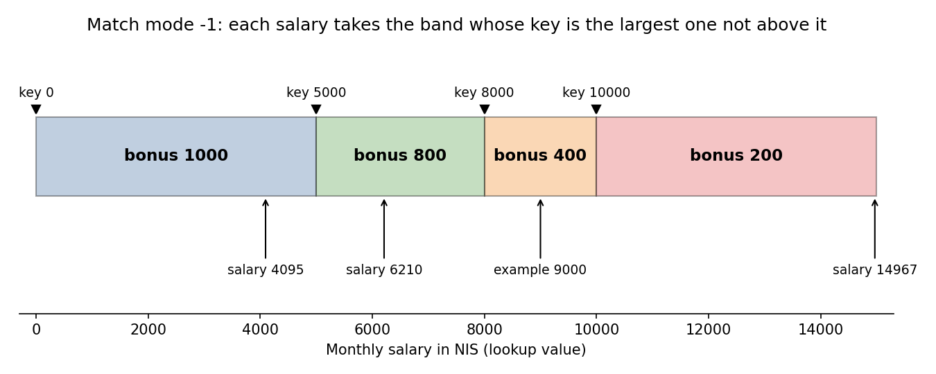
Real rows fromemployees
Employee Salary (NIS) Key chosen Bonus Salary + Bonus Gadi Guri (row 2) 6210 5000 800 7010 Lilach Argov (row 3) 4095 0 1000 5095 Avi Nathanson (row 4) 6066 5000 800 6866 Tal Dean (row 5) 12060 10000 200 12260 Hanney Pinchasof (row 8) 8851 8000 400 9251
I recomputed the bands in Python for all 200 employees: every stored bonus matches the rule. The distribution is 26 people at 1000, 76 at 800, 47 at 400 and 51 at 200, summing to NIS 115,800 in total bonuses.
3.3 Match modes compared
match_mode |
Behaviour | Typical use |
|---|---|---|
0 |
exact only, else not found | IDs, names, codes |
-1 |
exact, else the next smaller | bands where the table lists the lower limit of each band (this lecture) |
1 |
exact, else the next larger | bands where the table lists the upper limit |
2 |
wildcard (*, ?) |
partial text matches |
Choosing between -1 and 1Ask whether your table lists where each band starts or where it ends. A table that starts at 0, 5000, 8000, 10000 lists lower limits, so you step down to the key:
-1. If it listed 4999, 7999, 9999 and "no limit" you would step up:1.
Boundary behaviourA salary of exactly 5000 is an exact match to key
5000, so it earns 800, not 1000. That is why the teacher says "0-5000 (not including 5000)". No employee in the file earns exactly 5000, 8000 or 10000, so the boundary is not exercised by this data.
Common mistakes
- Leaving
-1off. The default exact match returns#N/Afor every salary that is not literally 0, 5000, 8000 or 10000.- Forgetting the lowest key. Without the row for
0, a salary below5000has nothing smaller to fall back to and gives#N/A.- Return array not aligned with the lookup array.
F217:F220andG217:G220both start at row 217.- Locking the ranges. The
$on both ranges is essential; the table must stay put whileJ2moves down.- Assuming a sort order. Unlike the old
VLOOKUP(..., TRUE), XLOOKUP with-1does not require the keys to be sorted. (The default search mode is linear, so it still works if the table is out of order; the table here is sorted ascending anyway.) This is reconstructed from how XLOOKUP is documented, not stated in the workbook.
Reconstructed from the workbookThe bonus formula is stored as a shared formula over
L3:L66,L67:L130and so on, which is just how Excel stores a formula that was filled down. Functionally it is one formula copied throughL2:L201.
4. INDEX and MATCH
The index&match sheet holds 178 students: first name (A), last name (B), full name (C) and five exercise grades (D to H, headed grade ex1 to grade ex5).
The full name is built by joining text:
=A2&" "&B2
The & operator concatenates; " " inserts a space. So Gadi and Guri become Gadi Guri. This gives a single column to search on.
First rows of the sheet, exactly as in the file:
| First Name | Last Name | full name | grade ex1 | grade ex2 | grade ex3 | grade ex4 | grade ex5 |
|---|---|---|---|---|---|---|---|
| Gadi | Guri | Gadi Guri | 49 | 8 | 31 | 43 | 46 |
| Lilach | Argov | Lilach Argov | 95 | 2 | 60 | 33 | 53 |
| Avi | Nathanson | Avi Nathanson | 49 | 52 | 59 | 44 | 41 |
| Tal | Dean | Tal Dean | 48 | 46 | 36 | 80 | 41 |
| Maayan | Shabbat | Maayan Shabbat | 54 | 52 | 49 | 68 | 8 |
4.1 The two building blocks
MATCH answers "in which position is it?" and returns a number.
=MATCH(lookup_value, lookup_array, [match_type])
INDEX answers "what is at this position?" and returns the cell content.
=INDEX(array, row_number, [column_number])
Together: MATCH finds the row and the column, INDEX reads the cell where they meet. That makes a two-way lookup: pick the row by student and the column by exercise.
4.2 The class example: a student's grade on one exercise
An input panel sits in K2:L4:
| Cell | Label | Content |
|---|---|---|
K2, L2 |
name |
Zvia Mizrahi (typed) |
K3, L3 |
ex |
grade ex5 (typed) |
K4, L4 |
grade |
formula below |
Step 1, the row position:
=MATCH(L2,C1:C179,0)
returns 34 (cell N2). Zvia Mizrahi is the 34th entry counted from C1.
Step 2, the column position:
=MATCH(L3,C1:H1,0)
returns 6 (cell N3). Counted from C1, the columns are full name (1), grade ex1 (2), grade ex2 (3), grade ex3 (4), grade ex4 (5), grade ex5 (6).
Step 3, combine with INDEX and a pass/fail test:
=IF(INDEX(C1:H179,MATCH(L2,C1:C179,0),MATCH(L3,C1:H1,0))<60,"FAIL",INDEX(C1:H179,MATCH(L2,C1:C179,0),MATCH(L3,C1:H1,0)))
(the workbook has extra brackets around each INDEX; they change nothing.)
Row 34 and column 6 of C1:H179 is H34, which holds 38. Since 38 is below 60 the cell shows FAIL.
| Student | Exercise | MATCH row | MATCH column | Grade | Shown |
|---|---|---|---|---|---|
| Zvia Mizrahi | grade ex5 | 34 | 6 | 38 | FAIL |
The position-alignment ruleThe
MATCHranges and theINDEXarray must start in the same row and column. All ofC1:C179,C1:H1andC1:H179start atC1, so position 34 means row 34 of the sheet and position 6 means columnH. If INDEX started atD2while MATCH counted fromC1, every answer would be shifted. An easy way to stay safe is to anchor everything at the header row and header column.
Why the0in MATCH
MATCH(..., 0)is exact match. Names and exercise labels are text, so you almost always want0. A1(default) assumes sorted data and can return a wrong row without any error.
The IF Function wrapper repeats the long INDEX/MATCH twice, once for the test and once for the value. This works but is hard to read; see Lec_02-IF Statements & Logical Functions for the IF logic.
Common mistakes
- MATCH returns the first match only. If two students shared a full name, the second would never be found; use a unique key such as an ID where possible.
- Typing
Zvia Mizrahiwith two spaces, or a trailing space, gives#N/A.- A name that is not in the list gives
#N/Afor the whole formula.
4.3 XLOOKUP versus INDEX and MATCH
| XLOOKUP | INDEX and MATCH | |
|---|---|---|
| Functions needed | one | two combined |
| Lookup direction | any (left or right of the return) | any |
| Default match | exact | MATCH defaults to approximate, so write 0 |
| Not found | built-in if_not_found |
wrap in IFERROR or IF |
| Returns several columns | yes (spills) | one cell per formula |
| Two-way (row and column) lookup | needs nesting two XLOOKUPs | natural |
| Availability | newer Excel only | every version |
Rule of thumb from this workbook: use XLOOKUP for a "find the row, return a column" lookup; use INDEX and MATCH when the column also has to be found from a label, as with grade ex5.
5. A pivot in the same workbook (brief)
Sheet2 and Sheet3 are two Pivot Tables built on employees!A1:N201, so they include the new Bonus column made by XLOOKUP. Full treatment is in Lec_07-Pivot Tables; here, just what they show.
Sheet2: rows areBranchthenLast Name, values areSum of Monthly Salary in NIS,Sum of BonusandCount of First Name. Totals, for example:
| Group | Sum of Monthly Salary in NIS | Sum of Bonus | Count of First Name |
|---|---|---|---|
| Tiberias Total | 168992 | 12400 | 21 |
| Grand Total | 1622904 | 115800 | 200 |
Sheet3: a one-cell pivot,Sum of Monthly Salary in NIS=1622904.
I confirmed these totals independently from the employees rows: Tiberias has 21 employees with NIS 168,992 salary and NIS 12,400 bonus, and the grand totals are NIS 1,622,904 and NIS 115,800. The link to this lecture: the bonus summed in the pivot is not typed data, it is the result of the approximate-match XLOOKUP, which shows why lookups feed later analysis.
Summary
- A lookup takes a key, finds it in one range and returns the matching item from another range of the same size.
- XLOOKUP has the form
XLOOKUP(value, search_range, return_range, if_not_found, match_mode, search_mode). Useif_not_found(as"") to hide#N/A, and a widerreturn_rangeto spill several columns. - Lock lookup and return ranges with
$so they do not move when filled down. - Exact match (
0) is for IDs and names; match mode-1is for banded values: it takes the largest key that does not exceed the value. The bonus table (0, 5000, 8000, 10000) gives 1000, 800, 400, 200. - INDEX and MATCH splits the job:
MATCHfinds a position,INDEXreturns the cell at a row and column. Two MATCHes give a two-way lookup. - Keep MATCH and INDEX ranges starting from the same cell so positions agree.
- Lookups produce columns (
feedback,Bonus,Area) that pivots then summarise.
Related notes
- Excel for Data Analysis
- Lec_01-Sorting, Filters & Database Functions (the
employeestable) - Lec_02-IF Statements & Logical Functions (IF logic used around INDEX/MATCH)
- Lec_07-Pivot Tables
- Lec_08-VBA Macros