
Introduction & Treatment Effects
Introduction & Treatment Effects
Part of: Econometrics Lecture 01 — Applied Econometrics, Dr. Aluma Dembo Key concepts: Causal Inference, Treatment Effects, Panel Data, OLS Estimation, Hypothesis Testing, Dummy Variables
Course Context
What this course is aboutApplied Econometrics is about upgrading your toolkit for causal inference — not just running regressions, but knowing what to do and why. The concurrent Data Science course teaches the how in R; this course teaches the why.
Prerequisite: Introduction to Econometrics. OLS, t-tests, F-tests, and the classical assumptions A1–A5 are assumed.
Types of Datasets
| Type | Description | Example |
|---|---|---|
| Cross-sectional | Sample at a fixed point in time | Demographics & wages of every student this semester |
| Time series | Single unit measured over time | Per-capita GDP each year |
| Panel (longitudinal) | Same cross-section sampled over time | Your HW grades over the semester |
| Repeated cross-section | Different cross-sections over time | Metrics grades from each year's cohort |
Why this distinction mattersThe classical OLS assumptions (especially A3: independent errors) assume a fresh cross-section. Panel data breaks this — which is why we'll need fixed effects, clustered standard errors, and similar tools later in the course.
The Core Problem: Causal Inference
Research question framing: Does variation in X (exogenous) cause variation in Y (endogenous)?
        X  ───────▶  Y
    (exogenous)    (endogenous)
For this arrow to be causal, we need:
- X varies randomly / exogenously
- Variation in Y is the direct result of variation in X (not through some other channel)
Correlation ≠ CausationOLS gives you a statistical association. To interpret as causal, you need to rule out:
- Confounders — other things varying with X that also affect Y
- Reverse causality — Y causing X
- Selection — non-random assignment of X
Worked Example: Andreoni & Miller (2002) Dictator Game
The SetupA dictator is given tokens and decides how many to keep vs. pass to an anonymous partner. Tokens are worth points; points convert to money at $0.10/point.
Three of the rounds used:
- Round A: 60 tokens. Hold @ 1pt, Pass @ 1pt. (symmetric)
- Round B: 60 tokens. Hold @ 2pts, Pass @ 1pt. (self-payout is cheap)
- Round C: 60 tokens. Hold @ 1pt, Pass @ 2pts. (other-payout is cheap)
The Data (176 subjects, 528 obs)
| Variable | Meaning |
|---|---|
| Tokens kept for self (0–60) | |
| Points per token to self (1 or 2) | |
| Points per token to other (1 or 2) | |
| ∈ {0.5, 1, 2} | |
| Points to self / total points (0 to 1) |
Whypct.points.selfinstead ofchoice?
choiceis measured in tokens, but tokens are worth different points in different rounds. To compare behavior across rounds on a common scale, normalize to the share of points allocated to self.
Findings from the Raw Data (Round A only)
- 40.9% kept everything for themselves
- 33.5% divided equally
- Only 2.8% gave more than they kept
- Mean = 45.4, Median = 50, SD = 14.3
Strong bimodal distribution: most subjects are either pure selfish or pure equal-splitters.
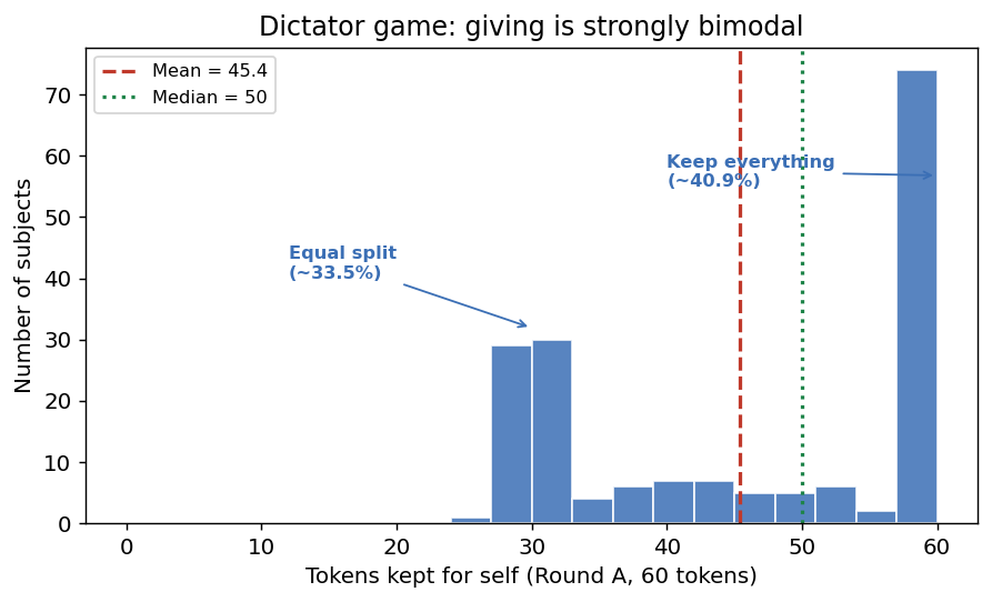
Why the mean is misleading hereThe data piles up at two points — keep everything (60 tokens) and split equally (30 tokens) — with very few people in between. The mean of 45.4 sits in a valley where almost no one actually is. This is exactly why a single summary number can hide the real behaviour, and why we model the response to price rather than just averaging tokens.
Regression Approaches
Option 1: Continuous Regressor
Null hypothesis: (no effect of relative price on behavior)
Interpretation:
- : when self-tokens pay more, dictators allocate more to self
- : dictators compensate by giving more to the other when self-tokens pay more
Results from R:
Estimate Std. Error t value Pr(>|t|)
(Intercept)       0.53090  0.02382  22.286  <2e-16 ***
ratio.price.self  0.17064  0.01801   9.476  <2e-16 ***
Residual std err: 0.258 on 526 df | R² = 0.146
F-stat: 89.79 on 1 and 526 DF, p-value: < 2.2e-16
t-test Review
Under classical assumptions A1–A5:
For :
With 526 d.f., the 5% t-critical value ≈ 1.96. Since , reject .
Option 2: Dummy Variables (Categorical)
Since ratio.price.self only takes three values {0.5, 1, 2}, treat it as categorical:
Where:
- if , else 0
- if , else 0
- Reference category: ratio = 1 (captured in )
Null hypothesis: (joint test → use F-test)
Results:
Estimate Std. Error t value Pr(>|t|)
(Intercept)        0.75748  0.01923  39.391 <2e-16 ***
ratio.price.half  -0.17855  0.02720  -6.566 1.25e-10 ***
ratio.price.two    0.09605  0.02720   3.532 0.000449 ***
F-statistic: 52.51 on 2 and 525 DF, p-value: < 2.2e-16
Interpretation:
- : When ratio = 1 (symmetric), dictators keep ~76% of points
- : When self-tokens are cheap (ratio = 0.5), share to self drops by 17.9pp
- : When self-tokens are expensive (ratio = 2), share to self rises by 9.6pp
F-test Review
For joint hypothesis :
- Restricted model:
- F-stat is a function of RSS in unrestricted vs. restricted models
- Distributed where = # restrictions
- Here , → F-critical ≈ 2.62
- → reject at 5%
The Panel Data Problem
Each of the 176 subjects appears 3 times (once per round). The 528 observations are not independent.
Which assumptions does this violate?
| Assumption | Statement | Violated? |
|---|---|---|
| A1 | ❌ Not violated | |
| A2 | ❌ Not violated | |
| A3 | for | ✅ Violated |
| A4 | ✅ Likely violated (errors correlated within individual) | |
| A5 | Normality of errors | ❌ Not directly |
ConsequenceStandard errors will be wrong (usually too small). t-stats and F-stats will look more significant than they really are. We'll fix this later with clustered SEs / fixed effects (week 10).
Quick-and-dirty fix: Subsample
Randomly pick 1 observation per subject → 172 obs, all independent.
With fewer obs, (ratio=2 dummy) is no longer individually significant, but the joint F-test still rejects — the effect is real.
Sensitivity via resampling ***You can repeat the random sub-sampling 1,000 times and check how the F-stat is distributed. In the data, 99.9% of subsamples have F > critical value → robust conclusion. (Not examinable — general knowledge.)
Extending the Analysis: Controlling for Income
The full experiment has 8 rounds varying both price ratio and total income (40, 60, 75, 80, 100 tokens).
  ratio.price.self ─┐
                    ├──▶  pct.points.self
  income ───────────┘
Research question: Does income affect behavior?
Approach 1: Full data + control variable
= marginal effect of +1 token of income, holding price ratio constant.
Result: , highly significant (t ≈ 6.5) but economically small relative to the price effect.
Approach 2: Subsample where price ratio = 1
Restrict to rounds 7, 8, 11 (all with ratio = 1). Regress pct.points.self on income alone.
Result: , not significant (p = 0.63). Treating income as categorical gives the same null.
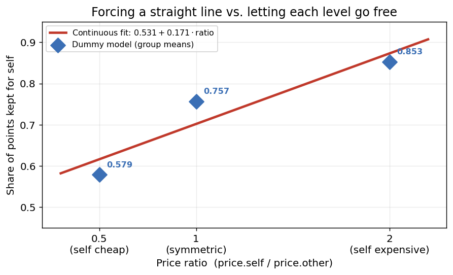
Continuous slope vs. flexible dummiesThe red line is the continuous model — it forces one straight-line slope across all three price ratios. The blue diamonds are the dummy model, which lets each ratio level take its own value (they're just the group means). Here the points sit close to the line, so the linear assumption is reasonable — but the dummy model is more flexible and would reveal any non-linearity (a level sitting off the line). With only three discrete values, dummies cost little and protect you from mis-specifying the functional form.
Key causal-inference lessonThe two approaches give similar answers only when the regression is correctly specified. Controlling (Approach 1) and subsampling (Approach 2) are two ways to isolate the effect of one variable while holding another constant — which strategy you use depends on sample size and which assumption you trust more.
Summary — What Lecture 1 Teaches
- Applied econometrics = causal inference. The regression coefficient is only causal if you've ruled out confounders and reverse causality.
- Build the causal diagram first. It tells you what to control for.
- Categorical regressors (dummies) are more flexible than forcing a continuous functional form — use dummies when the variable takes few discrete values.
- Panel data breaks A3 & A4. Naive OLS gives wrong SEs. Quick fix: subsample. Proper fix: comes later.
- To isolate the effect of X, either control for confounders explicitly, or subsample to rounds where only X varies.
Related Notes
- Next lecture: Lec_02-Linear Probability Model (LPM)
- Later: Lec_03-Logit & Probit Models — when the outcome is binary
- Foundational: OLS Estimation, Hypothesis Testing, Classical Assumptions A1-A5
- Coming up: Panel Data, Fixed Effects, Clustered Standard Errors